5
$\begingroup$

Suppose I have an transport equation with an initial conditions:

sol = NDSolve[{D[y[x, t], t] - 4 D[y[x, t], x] == 0, 
              y[x, 0] == 1/Sqrt[2 \[Pi]] Exp[-(x)^2/2], 
              y[10, t] == 0}, 
              y[x, t], {x, -10, 10}, {t, 0, 5}, 
              MaxStepSize -> 0.1];
Plot3D[Evaluate[y[x, t] /. sol], {x, -10, 10}, {t, 0, 2.5}, 
       PlotRange -> All]

enter image description here

Suppose the packet is actually a probability distribution. The packet is moving to the left, and at some later time, part of the probability density goes out of the left boundary such that the sum of the probability density in the domain [-10,10] is less than 1.

My question is, what should I do such that, at every time step, the sum of the probability density in the domain [-10,10] is 1?

$\endgroup$
6
  • $\begingroup$ Isn't it enough to normalize the result after solving the equation? $\endgroup$ Commented Apr 7, 2013 at 16:48
  • $\begingroup$ @belisarius, you are right if the mentioned question was all I wanted. However, I intended to break down a very complicated question into a simple one. The problem I really want to solve is one in which there are several (chemical) species reacting with each other, and the probability density of some species is going out of the domain through the left boundary, while some other species through the right boundary. Moreover, if I want to monitor the time evolution, normalizing at every step seems to be the only right way. $\endgroup$
    – wdg
    Commented Apr 7, 2013 at 17:08
  • 1
    $\begingroup$ Er… You mean you need to normalize y at the moment NDSolve gets the solution for the first time point and then solve the y at the next time point with this solution and so on? …Is it still a PDE-solving issue? $\endgroup$
    – xzczd
    Commented Apr 8, 2013 at 2:53
  • $\begingroup$ @xzczd, you are right. I believe it is a genuine PDE-solving problem. At least it involves NDSolve :-) $\endgroup$
    – wdg
    Commented Apr 8, 2013 at 3:58
  • $\begingroup$ Is the expected solution assumed to go towards left boundary and grow and grow approaching a dirac delta function? $\endgroup$
    – ssch
    Commented Apr 9, 2013 at 16:25

2 Answers 2

7
$\begingroup$

Here is the solution :

CRK4modified[]["Step"[rhs_, t_, h_, y_, yp_]] := 
 Module[{k0, k1, k2, k3, ampli},
  k0 = h yp;
  k1 = h rhs[t + h/2, y + k0/2];
  k2 = h rhs[t + h/2, y + k1/2];
  k3 = h rhs[t + h, y + k2];
  ampli = 
   If[t < 0.2, 1,  6.5 (* 6.5 : manually trimmed ! *)/Total[y]];
  {h, -y + ampli ((k0 + 2  k1 + 2  k2 + k3)/6 + y)}]
CRK4modified[___]["DifferenceOrder"] := 4
CRK4modified[___]["StepMode"] := Fixed

tEnd = 3;
sol20 = NDSolve[
         {  D[y[x, t], t] - 4 D[y[x, t], x] == 0, 
            y[x, 0] == 1/Sqrt[2 \[Pi]] Exp[-x^2/2],
            y[10, t] == 0}, 
         y,
         {x, -10, 10},
         {t, 0, tEnd},
         Method -> {MethodOfLines, 
            Method -> {"FixedStep", "StepSize" -> 0.02,Method -> CRK4modified},
            TemporalVariable -> t
            }
         ][[1]]

Plot3D[Evaluate[y[x, t] /. sol20], {x, -10, 10}, {t, 0, tEnd}, 
 PlotRange -> {Automatic, Automatic, {-0.1, 1}}]

enter image description here

The solution is based on the use of a do-it-yourself algorithm for solving the ODEs used by the PDE. I have token the example of the Runge-Kutta algorithm (CRK4) from the documentation (here, mathematica version 8) and modified it by dividing the solution-vector y (which values are > 0) by Total[y]. This maintains constant the area under the curve at each step.

This algorithm is intentionally effective only after t=0.2 second. This permits to adjust a multiplicative constant coefficient on Total[y] (6.5 here, try 8 to see the effectiveness of the algorithm, you will see that the height of the wave has a step at t=0.2)

Few details about the code of the modification of the Runge-Kutta algorithm CRK4 :

We want to divide the solution-vector by the surface of the curve. The correction factor is ampli = If[t < 0.2, 1, 6.5/Total[y]]; Total[y] is proportional to the surface, with a undetermined constant value that I have manually trimmed (the 6.5, which depends on the number of points of the spatial grid)

The term -y + ampli ((k0 + 2 k1 + 2 k2 + k3)/6 + y) in the increment of the solution-vector. As we want to multiply the vector (not the increment) by ampli, starting from the normal CRK4 increment (k0 + 2 k1 + 2 k2 + k3)/6, I have done a translation +y -> multiply by ampli-> back-translation (-y).

$\endgroup$
1
$\begingroup$

NOT a answer.
Here is a no successful attempt. Definitive ?

Mathematica has utilities that permit the user to manage time during temporal simulations. One can advance forward (and even backward) on a certain amount of time. Between theses intervals, I hope it should be possible to change the data.

It is documented in http://reference.wolfram.com/mathematica/tutorial/NDSolveStateData.html#93858351.

I currently use Mathematica 8.0.4., but the functionality I use here are old (maybe Version 5). It is possible that I miss a more recent functionality.

Here is a prolog to this simulation :

ndssdata = First[NDSolve`ProcessEquations[{
     D[y[x, t], t] - 4 D[y[x, t], x] == 0,
     y[x, 0] == 1/Sqrt[2 \[Pi]] Exp[-(x)^2/2],
     y[10, t] == 0
     },
   y,
   {x, -10, 10},
   {t, 0, 100}, MaxStepSize -> 0.01, 
   Method -> {MethodOfLines, TemporalVariable -> t}]]

then one can simulate the first 1.1 seconds :

NDSolve`Iterate[ndssdata, 1.1]

here is the code to see the result :

ndsol = NDSolve`ProcessSolutions[ndssdata]
Plot3D[Evaluate[y[x, t] /. ndsol], {x, -10, 10}, {t, 0, 1.1}, 
 PlotRange -> All]
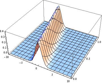
enter image description here

We can get the actual data from inside the simulator :

actualData=ndssdata@"SolutionVector"["Forward"];
ListPlot[actualData]
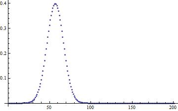
enter image description here

It seems that we can modify them, for example multiply them by 2 :

    Unprotect[NDSolve`StateData]
    ndssdata@"SolutionVector"["Forward"]= 2 ndssdata@"SolutionVector"["Forward"]
    ndssdata@"SolutionDerivativeVector"["Forward"]= 2 ndssdata@"SolutionDerivativeVector"
["Forward"]
    Protect[NDSolve`StateData]

but it is not effective : ndssdata@"SolutionVector"["Forward"] is not modified

EDIT

At the moment, it seems that to write in ndssdata@"SolutionVector"["Forward"]is not a solution.

If one want to stop the simulation, change the data, and resume the simulation, there is the possibility to use NDSolve``ReInitialize :

newstate = 
 First @ NDSolve`Reinitialize[
   ndssdata, {y[x, 0] == 2((ndsol[[1, 2]])[x, 2])}] (* 2="normalisation"*)

NDSolve`Iterate[newstate, 2]

Result :

ndsolnew = NDSolve`ProcessSolutions[newstate]
Plot3D[Evaluate[y[x, t] /. ndsolnew], {x, -10, 10}, {t, 0, 2}, 
 PlotRange -> All]
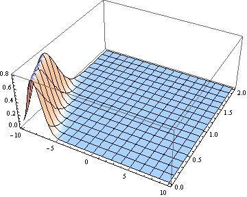
continuation of the simulation

we see the continuation of the simulation.

Not very good because :
- the time reset to 0 at every ReInitilization
- not applicable to each step

We can view the junction of the two parts with the following code (merge the whole + time of first simulation elongated to 2 seconds + no factor 2):

(* part 1 : *)
ndssdata = 
  First[NDSolve`ProcessEquations[  
      {  D[y[x, t], t] - 4 D[y[x, t], x] == 0,
         y[x, 0] == 1/Sqrt[2 \[Pi]] Exp[-(x)^2/2],
         y[10, t] == 0},  
      y,
      {x, -11, 10},
      {t, 0, 100},
      MaxStepSize -> 0.01,
      Method -> {MethodOfLines, TemporalVariable -> t}
      ]];
NDSolve`Iterate[ndssdata, 2]
ndsol = NDSolve`ProcessSolutions[ndssdata]
gr1 = Plot3D[Evaluate[y[x, t] /. ndsol],
                {x, -10, 3},{t, 0, 2}, 
                PlotRange -> All,PlotStyle -> Specularity[White, 5]];
tEndPartOne = Last[ndssdata @ "CurrentTime"];  

(* part 2 : *)
newstate = 
 First@NDSolve`Reinitialize[
   ndssdata,  
   {y[x, tEndPartOne] == ((ndsol[[1, 2]])[x, 2])}
   ] 
NDSolve`Iterate[newstate, 3.7]
ndsolnew = NDSolve`ProcessSolutions[newstate]
gr2 = Plot3D[Evaluate[y[x, t] /. ndsolnew],
             {x, -10, 3},{t, 2, 3.7}, 
             PlotRange -> All];  

(* whole :*)
Show[gr1, gr2]
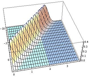
enter image description here

$\endgroup$
6
  • $\begingroup$ It's strange that basic manipulation to SolutionVector does not work... Isn't it supposed to be an "ordinary" variable? $\endgroup$
    – wdg
    Commented Apr 8, 2013 at 9:47
  • $\begingroup$ @wdg I'm not used in object programming. Maybe the problem is very basic. I think that ndssdata@"SolutionVector"["Forward"] is a field that can be set with =. $\endgroup$
    – andre314
    Commented Apr 8, 2013 at 13:00
  • $\begingroup$ @wdg It seems that ndssdata@"SolutionVector"["Forward"]is not modifiable (no example in documentation). Nevertheless, I succeed in modifying data and resume the simulation with NDSolve`Reinitialize. The problem will be that time return to 0 at every reinitialization. $\endgroup$
    – andre314
    Commented Apr 9, 2013 at 13:28
  • $\begingroup$ Reinitialize seems to be a nice work-around. Unfortunately, we would have to "glue" the solution manually, and there may be notable discontinuities in the solution. $\endgroup$
    – wdg
    Commented Apr 11, 2013 at 3:56
  • $\begingroup$ @wdg There are no discontinuity (see figure I have just added). Maybe you have tried to glue the two first part of the answer. Warning : they are not in a "continuous" time interval (first : [0,1.1], second : [2,4]. There was also a factor 2 to simulate renormalisation. $\endgroup$
    – andre314
    Commented Apr 11, 2013 at 9:10

Your Answer

By clicking “Post Your Answer”, you agree to our terms of service and acknowledge you have read our privacy policy.

Not the answer you're looking for? Browse other questions tagged or ask your own question.