21
$\begingroup$

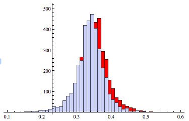
I am plotting two histograms on the same graph:

g1 = Histogram[bc, ChartStyle -> {Red}]
g2 = Histogram[bcx]
Show[g1, g2, PlotRange -> {{0.1, 0.6}, All}]

enter image description here

But I would like the plots to overlap so that they are "see-through" and I can compare them. I've been trying with

ChartStyle -> {"Overlapped"}

which hasn't been working.

$\endgroup$

4 Answers 4

22
$\begingroup$

First method

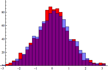
You could make the one in front partially transparent:

bc = RandomVariate[NormalDistribution[], 1000];
bcx = RandomVariate[NormalDistribution[], 1000];

g1 = Histogram[bc, ChartStyle -> {Red}];
g2 = Histogram[bcx, ChartStyle -> {Directive[Blue, Opacity[.5]]}];
Show[g1, g2, PlotRange -> All]

Mathematica graphics

Direct method

The same effect can be achieved by plotting the two distributions in the same plot directly:

Histogram[{bc, bcx}, ChartStyle -> {Red, Blue}]
$\endgroup$
2
  • 1
    $\begingroup$ Why lead with the more complex solution?! $\endgroup$ Commented Feb 24, 2012 at 21:54
  • 2
    $\begingroup$ @BrettChampion the second one didn't occur to me until after I finished writing the more complex solution. $\endgroup$
    – Heike
    Commented Feb 24, 2012 at 21:59
32
$\begingroup$

Doesn't Histogram do this already?

data1 = RandomReal[NormalDistribution[0, 1], 500];
data2 = RandomReal[NormalDistribution[1, 1.5], 500];

Histogram[{data1, data2}]
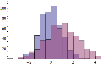
Mathematica graphics


Version 7 doesn't have HistogramDistribution as shown by Andy Ross. Here is an alternative:

Histogram[{data1, data2},
  BaseStyle  -> FaceForm[None],
  ChartStyle -> {EdgeForm[{Thick, Red}], EdgeForm[{Thick, Blue}]}
]
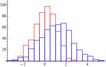
Mathematica graphics


jmlopez asked for a method without the vertical lines. Here is one. The replacement may be a bit fragile. Andy's method is safer for version 8 users.

Update: modified to work in Mathematica 10 as well.

h =
 Histogram[{data1, data2},
   ChartStyle -> (Directive[#, AbsoluteThickness[3]] & /@ {Red, Blue}),
   PerformanceGoal -> "Speed"
 ];

h2 =
 Histogram[{data1, data2},
   ChartStyle -> {{Red, Blue}, Directive[Opacity[0.1], EdgeForm[]]}
 ];

hline = h /. rec : {({{_Rectangle}} | {}) ..} :>
  Line[  Flatten[rec, 2] /. _[{x_, y_}, {X_, Y_}, ___] :> Sequence[{x, Y}, {X, Y}]  ];

Show[hline, h2]
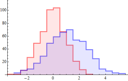
Mathematica graphics


kjo pointed out that my method fails when bars have a height of zero. The simplest fix I can think of is to avoid zero-height bars (which are not drawn, the source of the problem) by using a small offset value for the hspec function.

hfn = $MachineEpsilon + #2 &;

h = Histogram[{data1, data2}, {0.1}, hfn, 
  ChartStyle -> (Directive[#, AbsoluteThickness[3]] & /@ {Red, Blue}), 
  PerformanceGoal -> "Speed"]

h2 = Histogram[{data1, data2}, {0.1}, hfn, 
  ChartStyle -> {{Red, Blue}, Directive[Opacity[0.1], EdgeForm[]]}]

hline = h /. 
   rec : {({{_Rectangle}} | {}) ..} :> 
    Line[Flatten[rec, 2] /. _[{x_, y_}, {X_, Y_}, ___] :> Sequence[{x, Y}, {X, Y}]];

Show[hline, h2]
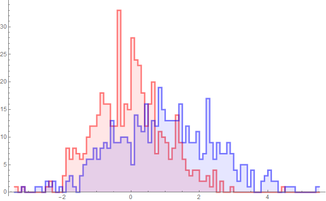
enter image description here

$\endgroup$
5
  • $\begingroup$ Is there a way to get rid of the middle lines? And get something like this on the second example. I like how they just set the Apperance to Transparent and its done. $\endgroup$
    – jmlopez
    Commented Jun 4, 2012 at 22:47
  • 3
    $\begingroup$ I feel that it is a little absurd how there is tons of examples of how to use Histogram and yet there is no option to do what you just did in the update. All it really is is a line plot connecting points with the fill axis property. Anyway, thank you Mr. Wizard. $\endgroup$
    – jmlopez
    Commented Jun 5, 2012 at 7:46
  • 1
    $\begingroup$ There's a problem with the histogram outlining scheme at the end (last plot), when the histogram contains empty bins (not an uncommon situation, especially towards the tails). To elicit this condition, just add a narrow bin width specification (e.g. {0.1}) as a second argument to the Histogram expressions. $\endgroup$
    – kjo
    Commented May 18, 2017 at 18:01
  • 1
    $\begingroup$ @kjo I think I found a relatively simple fix; please take a look and test it for me. $\endgroup$
    – Mr.Wizard
    Commented May 21, 2017 at 6:03
  • $\begingroup$ Your fix is very elegant I think, and it works beautifully. A couple of thoughts. Since the offset added by the hspec function (hfn) is so small, one could omit it from the second histogram (h2). In fact, if one has some time to kill, one could even set hfn = offset + #2 &, for some arbitrary positive integer offset, and then change the last subexpression in hline from Sequence[{x, Y}, {X, Y}] to Sequence[{x, Y - offset}, {X, Y - offset}]. (A probably useless embellishment.) $\endgroup$
    – kjo
    Commented May 23, 2017 at 12:18
23
$\begingroup$

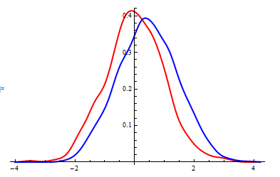
You also have the option of SmoothHistogram.

data1 = RandomVariate[NormalDistribution[0, 1], 10^3];
data2 = RandomVariate[NormalDistribution[.4, 1], 10^3];

SmoothHistogram[{data1, data2}, 
 PlotStyle -> {{Thick, Red}, {Thick, Blue}}]

enter image description here

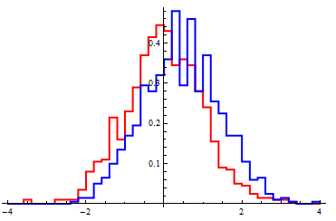
Or using one of the nonparametric distributions HistogramDistribution...

Plot[Evaluate[{PDF[HistogramDistribution[data1], x], 
   PDF[HistogramDistribution[data2], x]}], {x, -4, 4}, 
 Exclusions -> None, PlotPoints -> 100, 
 PlotStyle -> {{Thick, Red}, {Thick, Blue}}]

enter image description here

$\endgroup$
4
$\begingroup$

For g2 you should be able to change the definition to:

g1 = Histogram[bcx, ChartStyle -> Opacity[0.50, Blue]]

To get the front histogram to be more transparent. Fiddle around with the 0.50 to get it to look the way that you want.

$\endgroup$

Your Answer

By clicking “Post Your Answer”, you agree to our terms of service and acknowledge you have read our privacy policy.

Not the answer you're looking for? Browse other questions tagged or ask your own question.