Mathematica vs. MATLAB: why am I getting different results for PDE with non-constant boundary condition?

Question

I am trying to solve the same PDE in Mathematica and MATLAB, $\nabla^2\phi=0$ where $\phi=f(x,y)$ It has a Dirichlet boundary condition on the left, a section of non-constant Neumann boundary condition on the right and zero flux everywhere else. The non-constant boundary condition is defined by $\frac1{\sigma_i}\left(\frac{\sigma_i}{4e}\frac{\partial \mu}{\partial x}-I_e\right)$ where $\mu=f(x,y)$ was previously solved for and all other variables are constants. I have developed code for to solve this PDE in both Mathematica and MATLAB however, they do not produce the same results, and I do not know which code is incorrect.

Below is the full Mathematica code:

Needs["NDSolve`FEM`"]
e = 1.60217662*10^-19;
sigi = 18; 
F = 96485; 
n = -0.02; 
c = 1;
pO2 = 1.52*10^-19;
Ie = -(2*F)*(c*pO2^n);
mu2 = -5.98*10^-19;
l = 10*10^-6;
y1 = 0.01;
y2 = 0.0025;
y3 = 0.0075;
meshRefine[vertices_, area_] := area > 10^-12;
mesh = ToElementMesh[
   DiscretizeRegion[ImplicitRegion[True, {{x, 0, l}, {y, 0, y1}}]], 
   MeshRefinementFunction -> meshRefine];
bcmu = {DirichletCondition[mu[x, y] == 0, (x == 0 && 0 < y < y1)], 
  DirichletCondition[
   mu[x, y] == 
    mu2, (x == l && 
     y2 < y < y3)]};
solmu = NDSolve[{Laplacian[mu[x, y], {x, y}] == 
    0 + NeumannValue[0, 
      y == 0 || 
       y == y1 || (x == l && 0 <= y <= y2) || (x == l && 
         y3 <= y <= y1)], bcmu}, 
  mu, {x, y} \[Element] mesh];
bcphi = DirichletCondition[phi[x, y] == 0, (x == 0 && 0 < y < y1)];
A = (Ie - sigi/(4*e)*(D[mu[x, y] /. solmu, x] /. x -> l))/(-sigi);
solphi = NDSolve[{Laplacian[phi[x, y], {x, y}] == 
     0 + NeumannValue[0, 
       y == 0 || 
        y == y1 || (x == l && 0 <= y <= y1) || (x == l && 
          y3 <= y <= y1)] + 
      NeumannValue[-A[[1]], x == l && y2 < y < y3], bcphi}, 
   phi, {x, y} \[Element] mesh];
DensityPlot[phi[x, y] /. solphi, {x, 0, l}, {y, 0, y1}, 
 PlotLabel -> "Phi vs. x and y", PlotLegends -> Automatic]

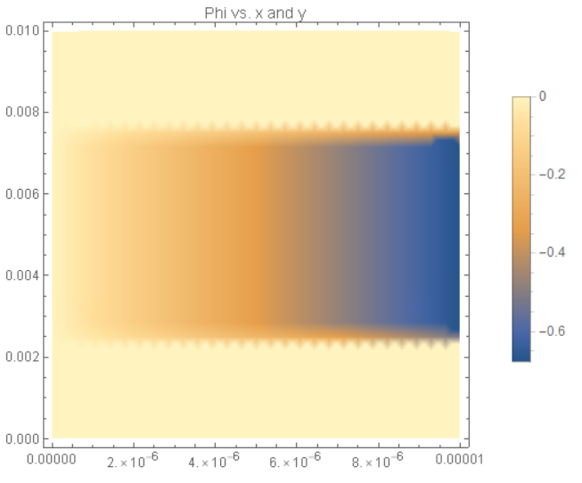
The code produces this result for phi:

And here is the MATLAB code:

% Define constants
e = 1.60217662*10^-19;
sigi = 18;
F = 96485;
n = -0.02;
c = 1;
pO2 = 1.52*10^-19;
Ie = -(2*F)*(c*pO2^n);
mu2 = -5.98*10^-19;
l = 10*10^-6;
y1 = 0.01;
y2 = 0.0025;
y3 = 0.0075;

% Rectangle is code 3, 4 sides, followed by x-coordinates and then y-coordinates
R1 = [3,4,0,l,l,0,0,0,y2,y2]';
R2 = [3,4,0,l,l,0,y2,y2,y3,y3]';
R3 = [3,4,0,l,l,0,y3,y3,y1,y1]';
geom = [R1,R2,R3];
% Names for the two geometric objects
ns = (char('R1','R2','R3'))';
% Set formula
sf = 'R1+R2+R3';
% Create geometry
g = decsg(geom,sf,ns);

% Create mu geometry model
mumodel = createpde;
geometryFromEdges(mumodel,g);

% Apply boundary conditions
applyBoundaryCondition(mumodel,'dirichlet','Edge',8,'u',0);
applyBoundaryCondition(mumodel,'dirichlet','Edge',9,'u',0);
applyBoundaryCondition(mumodel,'dirichlet','Edge',10,'u',0);
applyBoundaryCondition(mumodel,'dirichlet','Edge',6,'u',mu2);
applyBoundaryCondition(mumodel,'neumann','Edge',1,'g',0);
applyBoundaryCondition(mumodel,'neumann','Edge',3,'g',0);
applyBoundaryCondition(mumodel,'neumann','Edge',4,'g',0);
applyBoundaryCondition(mumodel,'neumann','Edge',2,'g',0);
applyBoundaryCondition(mumodel,'neumann','Edge',5,'g',0);
applyBoundaryCondition(mumodel,'neumann','Edge',7,'g',0);

% Solve PDE for mu
specifyCoefficients(mumodel,'m',0,'d',0,'c',1,'a',0,'f',0);
generateMesh(mumodel,'Hmax',l);
solmu = solvepde(mumodel);

% Create phi geometry model
phimodel = createpde;
geometryFromEdges(phimodel,g);

% Make sure initial condition is suitable
setInitialConditions(phimodel,0);
setInitialConditions(phimodel,-0.7,'Edge',6);

% Define nonconstant Neumann boundary condition
bcfun = @(location,state)(sigi/(4*e)*evaluateGradient(solmu,l,location.y)-Ie)/sigi;

% Apply boundary conditions
applyBoundaryCondition(phimodel,'dirichlet','Edge',8,'u',0);
applyBoundaryCondition(phimodel,'dirichlet','Edge',9,'u',0);
applyBoundaryCondition(phimodel,'dirichlet','Edge',10,'u',0);
applyBoundaryCondition(phimodel,'neumann','Edge',6,'g',bcfun);
applyBoundaryCondition(phimodel,'neumann','Edge',1,'g',0);
applyBoundaryCondition(phimodel,'neumann','Edge',3,'g',0);
applyBoundaryCondition(phimodel,'neumann','Edge',4,'g',0);
applyBoundaryCondition(phimodel,'neumann','Edge',2,'g',0);
applyBoundaryCondition(phimodel,'neumann','Edge',5,'g',0);
applyBoundaryCondition(phimodel,'neumann','Edge',7,'g',0);

% Solve PDE for phi and plot results
specifyCoefficients(phimodel,'m',0,'d',0,'c',1,'a',0,'f',0);
generateMesh(phimodel,'Hmax',l);
solphi = solvepde(phimodel);
phi = solphi.NodalSolution;
pdeplot(phimodel,'XYData',phi)
title('Phi vs. x and y')
xlabel('x-position')
ylabel('y-position')

The MATLAB code produces this as the results for phi:

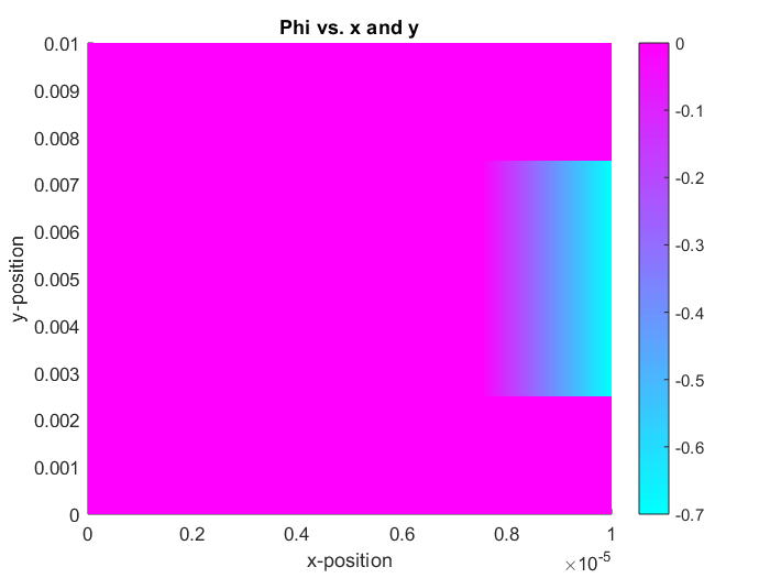
Which code is correct? Where is the error?

Answer 1

As @Henrik Schumacher points out, you have a very high aspect ratio (1000:1) domain. It is always conducive to conduct a dimensional analysis of your system. In the OP case, the dimensional analysis would show that the problem is essentially 1D in the $x$ direction.

I will use the subscript $d$ to indicate that the variable has dimensions. First, we can rewrite the Laplacian operator for $\mu_d$ in coefficient form.

$$ - {\nabla ^2}{\mu _d} = \nabla \cdot \left( {\begin{array}{*{20}{c}} { - 1}&0 \\ 0&{ - 1} \end{array}} \right)\nabla {\mu _d} = 0$$

We will use the following dimensionless variables:

$$x = \frac{{{x_d}}}{L};y = \frac{{{y_d}}}{H};\mu = \frac{{{\mu _d}}}{{{\mu _2}}}$$

Making the appropriate substitutions, we arrive at the dimensionless version of $\mu$ equation

$$\nabla \cdot \left( {\begin{array}{*{20}{c}} { - {{\left( {\frac{1}{L}} \right)}^2}}&0 \\ 0&{ - {{\left( {\frac{1}{H}} \right)}^2}} \end{array}} \right)\nabla \mu = 0\left\| {{L^2}} \right.$$

$$\nabla \cdot \left( {\begin{array}{*{20}{c}} { - 1}&0 \\ 0&{ - {{\left( {\frac{L}{H}} \right)}^2}} \end{array}} \right)\nabla \mu = 0$$

In dimensionless form, the y component of the diffusion coefficient matrix is $10^6$ smaller than x component and can effectively be ignored. The "correct" model should show a linear gradient along the x-direction for either a Dirichlet or flux boundary condition. The Mathematica result more accurately captures this linear gradient.

As a practical matter, your problem requires differentiation along a boundary that has a discontinuous jump in nodal values. Getting that to behave could be quite challenging. One will require very fine meshing near the discontinuity to mitigate the differentiation problems. I will demonstrate on the $\mu$ equation.

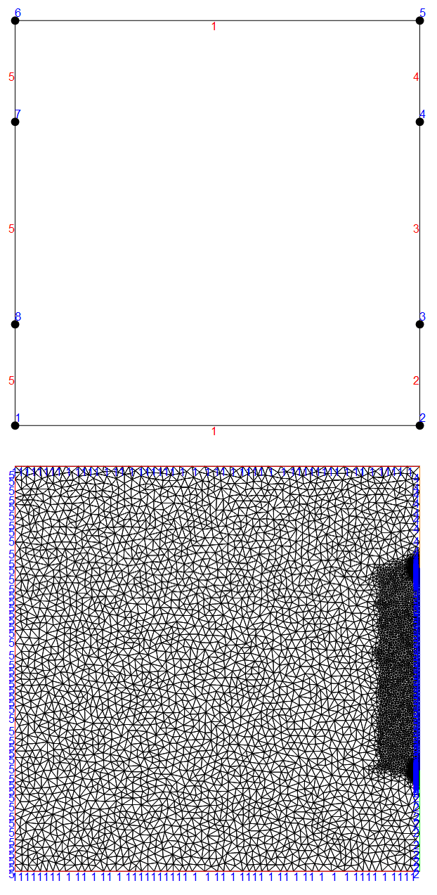
First, let's set up a mesh with very high refinement near the discontinuities and medium refinement between the discontuities in Dirichlet conditions.

pts = {{0, 0}, {1, 0}, {1, 1/4}, {1, 3/4}, {1, 1}, {0, 1}, {0, 
    3/4}, {0, 1/4}};
incidents = Partition[FindShortestTour[pts][[2]], 2, 1];
markers = {1, 2, 3, 4, 1, 5, 5, 5};
bcEle = {LineElement[incidents, markers]};
bmesh = ToBoundaryMesh["Coordinates" -> pts, 
   "BoundaryElements" -> bcEle];
Show[
 bmesh["Wireframe"["MeshElement" -> "BoundaryElements", 
   "MeshElementMarkerStyle" -> Red]],
 bmesh["Wireframe"["MeshElement" -> "PointElements", 
   "MeshElementStyle" -> Directive[PointSize[0.02]],
   "MeshElementIDStyle" -> Blue
   ]]]
mrf = With[{rmf = 
     RegionMember[
      Region@RegionUnion[Disk[{1, 0.25}, 0.025], 
        Disk[{1, 0.75}, 0.025]]]}, 
   Function[{vertices, area}, 
    Block[{x, y}, {x, y} = Mean[vertices]; 
     Which[rmf[{x, y}], area > 0.000025/258,
      (x > 0.9) && (0.25 <= y <= 0.75), area > 0.000025,
      True, area > 0.00025]]]];
mesh = ToElementMesh[bmesh, MeshRefinementFunction -> mrf];
Show[mesh["Wireframe"],
 mesh["Wireframe"["MeshElement" -> "BoundaryElements", 
   "MeshElementMarkerStyle" -> Blue, 
   "MeshElementStyle" -> {Red, Green, Blue, Orange}]]]
Show[mesh["Wireframe"],
  mesh["Wireframe"["MeshElement" -> "PointElements", 
    "MeshElementMarkerStyle" -> Blue, 
    "MeshElementStyle" -> {Black, Green, Red, Orange}]]];

You can see the mesh is quite refined in the desired areas. Now, set up the pde system for dimensionless $\mu$ and solve.

op = ( Inactive[
     Div][({{-1, 0}, {0, -0.001^2}}.Inactive[Grad][
       mu[x, y], {x, y}]), {x, y}]);
pde = op == 0;
dcmu1 = DirichletCondition[mu[x, y] == 0, ElementMarker == 5];
dcmu2 = DirichletCondition[mu[x, y] == -1, ElementMarker == 3];
mufun = NDSolveValue[{pde, dcmu1, dcmu2}, mu, {x, y} \[Element] mesh];
ContourPlot[mufun[x, y], {x, y} \[Element] mesh, 
 ColorFunction -> "TemperatureMap", AspectRatio -> Automatic, 
 PlotRange -> All, Contours -> 20, PlotPoints -> All]
DensityPlot[mufun[x, y], {x, y} \[Element] mesh, 
 ColorFunction -> "TemperatureMap", AspectRatio -> Automatic, 
 PlotRange -> {-1, 0}, PlotPoints -> All]
Plot[Evaluate[mufun[x, y] /. x -> 1], {y, 0, 1}, PlotPoints -> 200]
Plot[Evaluate[D[mufun[x, y], x] /. x -> 1], {y, 0, 1}, 
 PlotPoints -> 200, MaxRecursion -> 6]

Even with this level of refinement, the solution looks suspect near the boundary conditions. You can also see the spikes in the x derivative evaluated at the boundary.

In previous answers, I have used RegionProduct to construct Tensor Product Grids to create mapped quad meshes that can provide great refinement in regions of interest. I will show an example workflow that creates high refinement with mesh growth near the discontinuous Dirichlet conditions. First define some helper functions to create the mapped mesh.

(* Define Some Helper Functions For Structured Quad Mesh*)
pointsToMesh[data_] :=
  MeshRegion[Transpose[{data}], 
   Line@Table[{i, i + 1}, {i, Length[data] - 1}]];
unitMeshGrowth[n_, r_] := 
 Table[(r^(j/(-1 + n)) - 1.)/(r - 1.), {j, 0, n - 1}]
unitMeshGrowth2Sided [nhalf_, r_] := (1 + Union[-Reverse@#, #])/2 &@
  unitMeshGrowth[nhalf, r]
meshGrowth[x0_, xf_, n_, r_] := (xf - x0) unitMeshGrowth[n, r] + x0
firstElmHeight[x0_, xf_, n_, r_] := 
 Abs@First@Differences@meshGrowth[x0, xf, n, r]
lastElmHeight[x0_, xf_, n_, r_] := 
 Abs@Last@Differences@meshGrowth[x0, xf, n, r]
findGrowthRate[x0_, xf_, n_, fElm_] := 
 Abs@FindRoot[
    firstElmHeight[x0, xf, n, r] - fElm, {r, 1.0001, 100000}, 
    Method -> "Brent"][[1, 2]]
meshGrowthByElm[x0_, xf_, n_, fElm_] := 
 Chop@meshGrowth[x0, xf, n, findGrowthRate[x0, xf, n, fElm]]
reflectRight[pts_] := With[{rt = ReflectionTransform[{1}, {Last@pts}]},
  Union[pts, Flatten[rt /@ Partition[pts, 1]]]]
reflectLeft[pts_] := 
 With[{rt = ReflectionTransform[{-1}, {First@pts}]},
  Union[pts, Flatten[rt /@ Partition[pts, 1]]]]

Now, setup the mesh and solve the PDE system.

points = Union[meshGrowthByElm[0.25, 0, 75, 0.00001], 
   meshGrowthByElm[0.25, 0.5, 75, 0.00001]];
regy = pointsToMesh@reflectRight[points];
regx = pointsToMesh@Subdivide[0, 1, 50];
rp = RegionProduct[regx, regy]
crd = MeshCoordinates[rp];
inc = Delete[0] /@ MeshCells[rp, 2];
mesh = ToElementMesh["Coordinates" -> crd, 
   "MeshElements" -> {QuadElement[inc]}];
mesh["Wireframe"];
op = ( Inactive[
     Div][({{-1, 0}, {0, -0.001^2}}.Inactive[Grad][
       mu[x, y], {x, y}]), {x, y}]);
pde = op == 0;
dcmu1 = DirichletCondition[mu[x, y] == 0, x == 0];
dcmu2 = DirichletCondition[
   mu[x, y] == -1, (x == 1) && (0.25 <= y <= 0.75)];
mufun = NDSolveValue[{pde, dcmu1, dcmu2}, mu, {x, y} \[Element] mesh];
ContourPlot[mufun[x, y], {x, y} \[Element] mesh, 
 ColorFunction -> "TemperatureMap", AspectRatio -> Automatic, 
 PlotRange -> All, Contours -> 20, PlotPoints -> All]
DensityPlot[mufun[x, y], {x, y} \[Element] mesh, 
 ColorFunction -> "TemperatureMap", PlotPoints -> All, 
 AspectRatio -> Automatic, PlotRange -> All]
Plot[Evaluate[mufun[x, y] /. x -> 1], {y, 0, 1}, PlotPoints -> 200, 
 PlotLabel -> "mu on Right Boundary"]
Plot[Evaluate[D[mufun[x, y], x] /. x -> 1], {y, 0, 1}, 
 PlotPoints -> 200, MaxRecursion -> 6, 
 PlotLabel -> "X-Derivative mu on Right Boundary"]

As predicted by dimensional analysis, the problem is essentially 1 dimensional in the x direction. The x-derivative of $\mu$ is essentailly constant between $y=0.25$ and $y=0.75$.

To summarize, the OP Mathematica implementation looks more correct than their Matlab implementation. To achieve high accuracy, will require the appropriate meshing strategy.