LatticeData makes use of the abstract Mathematica Entity Lattice. This reflects the physical interpretation of lattices in solids. So it is in general translational. Translational is in general not periodic.
It depends on the task to be periodic. Visualization can not be periodic. To represent translational infinity usually the finite lattice graphic is cut off without showing blank space.
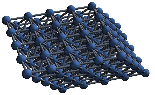
The first part shows the general how to create, generate points in the lattice-based on the basic Basis lattice cell from the class Bravais in the type Cubic.
It is rather unusual to use NearestNeighborGraph since interest is in the bounds inside the solid that are available for simulation of physical properties.
To represent a general function on these points this solution is useful in general: How to plot periodic function's graphic?. This is straight forward if the function is multiplative in the coordinates.
Since the atoms are small compared to interatomic distance a DiracDelta function is used for examples for electron movement. Mathematica has the newer function DiracComb. This shows there is extra effort internally necessary for doing periodic calculations such as integration, differentiations with periodic condition. It to shows that lattice implies only a finite range of cell contribute to the local field.
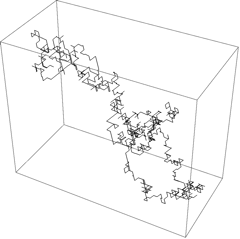
There is an example for random walk on a lattice in the Mathematica documentation: random walk in two and three dimensions. Random walk is an arbitrary one step after another. It can but does not mean reach every point or be space filling.
Together with this are various statistic functions available as built-ins.
The process ist two step:
data3d = RandomFunction[RandomWalkProcess[0.5], {0, 10^3}, 3];
and
Graphics3D[Line[Transpose@data3d["States"]], BoxRatios -> Automatic]

This is already Cubic from Bravais of the Entities realized in Mathematica.
To the part of the question: (I believe the lattice is centered at {0,0,0}, and the cell is extended by the 𝑛 and 𝑚 units from here -in case this is useful-)
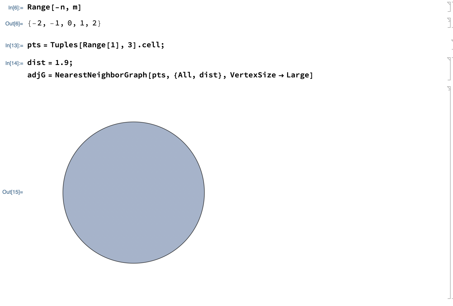
Reduce the Tuples[Range[-n, m], 3] to the minimum:
pts = Tuples[Range1, 3].cell;
dist = 1.9;
adjG = NearestNeighborGraph[pts, {All, dist}, VertexSize -> Large]

This shows that in and around the origin is a atom, edge what ever there should be. The basis cell spans into the positive quadrant. This is shown in complete with the basis vector of the Lattice.
The random walk process is implemented on infinite lattices as the documentation claims Random Walk Process. For the domain of statistic processes, the random walk is a foundation and therefore implemented in Mathematica itself.
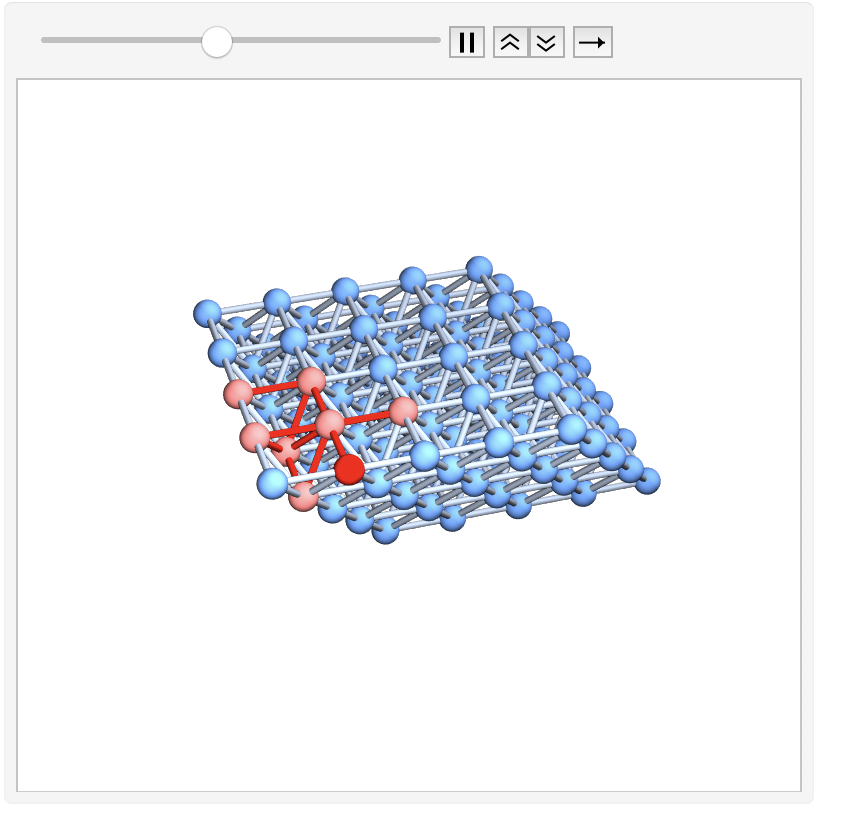
With this status it appears really often in mathematica.stackexchange.com. A nice solution is colorize 3d random walk of pi digits. The problem is, this are real numerical experiments and the Lattice for example for an overlay with Show large enough. So only little steps may be a good choice. This Generate random walk on a graph looks nice and offers best overview:
    Block[{graph = adjG, start, path},
 start = RandomChoice[VertexList[graph]];
 path = NestList[RandomChoice[AdjacencyList[graph, #]] &, start, 30];
 ListAnimate[
  Table[Graph[graph,
    VertexStyle ->
     Append[Map[Rule[#, Pink] &, Union[path[[1 ;; v]]]],
      path[[v]] -> Red],
    EdgeStyle ->
     Evaluate[(UndirectedEdge[#1, #2] -> Directive[Red, Thick]) & @@@
       Partition[path[[1 ;; v]], 2, 1]], VertexSize -> Large], {v,
    Length[path]}]]]
