1
$\begingroup$

I am trying to plot these graphics together. I tried with Plot and Show command but it doesn't work. Please help!

sol2 = NDSolve[{0.0099 u'[t] == v[t] - u[t]*v[t] + u[t] - 2 u[t]^2, 
   2.4892*10^(-5)*v'[t] == -v[t] - (u[t])*v[t] + 0.45*3, u[0] == 0.1, 
   v[0] == 0.2}, {u[t], v[t]}, {t, 0, 50}]
q1 = Plot[u[t] /. sol2, {t, 0, 1}, PlotStyle -> Red]
q2 = Plot[v[t] /. sol2, {t, 0, 1}, PlotStyle -> Blue]
Show[{q1, q2}]
$\endgroup$
4
  • $\begingroup$ It is actually working, the only issue is that the plot range for the Show command comes from the first plot. If you use Show[q1, q2, PlotRange -> {0.68, 0.81}] you should see both plots. However, they look like flat lines because the plot ranges are so different (look at the y-axis of the plots for q1 and q2). $\endgroup$
    – MassDefect
    Commented Nov 24, 2019 at 19:34
  • $\begingroup$ Thanks! Actually they are not so different - they are in the range (0.6,0.8). I cannot understand why the graphs are straight lines. $\endgroup$ Commented Nov 24, 2019 at 20:02
  • $\begingroup$ Look closely at the plot ranges of the individual plots. $\endgroup$
    – Bob Hanlon
    Commented Nov 24, 2019 at 20:17
  • $\begingroup$ The height of each graph is like 0.00001. When you scale the graph to show from 0.6 to 0.8, the height of each curve becomes very very small. $\endgroup$
    – MassDefect
    Commented Nov 25, 2019 at 3:09

1 Answer 1

2
$\begingroup$

There is not a one-size-fit-all solution for this, I think.

If you are more interested in comparing those functions on the same scale:

q1 = Plot[u[t] /. sol2, {t, 0, 1}, PlotStyle -> Red, PlotRange -> All];
q2 = Plot[v[t] /. sol2, {t, 0, 1}, PlotStyle -> Blue, 
   PlotRange -> All];
Show[{q1, q2}, PlotRange -> Full, ImageSize -> Scaled[0.6]]

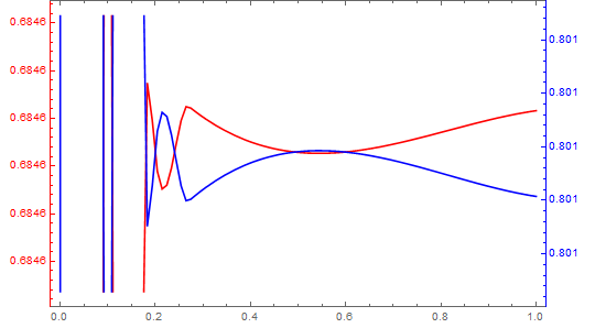
If you are interested in fine structure of those functions then this representation should be more helpful:

q1 = Plot[
   u[t] /. sol2, {t, 0, 1}
   , PlotStyle -> Red
   , ImagePadding -> {{45, 45}, {20, 0}}
   , Frame -> {True, True, True, False}
   , FrameStyle -> {Automatic, Red, Automatic, Automatic}
   , ImageSize -> Scaled[0.6]
   ];
q2 = Plot[
   v[t] /. sol2, {t, 0, 1}
   , PlotStyle -> Blue
   , ImagePadding -> {{45, 45}, {20, 0}}
   , Frame -> {False, False, False, True}
   , FrameTicks -> {{None, All}, {None, None}}
   , FrameStyle -> {Automatic, Automatic, Automatic, Blue}
   , ImageSize -> Scaled[0.6]
   ];
Overlay[{q1, q2}]
$\endgroup$
1
  • $\begingroup$ That is very useful! Thanks! $\endgroup$ Commented Nov 26, 2019 at 15:50

Your Answer

By clicking “Post Your Answer”, you agree to our terms of service and acknowledge you have read our privacy policy.

Not the answer you're looking for? Browse other questions tagged or ask your own question.