30
$\begingroup$

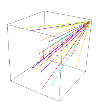
Consider a set of trajectories in 3D space, that possibly converge. By visualizing trajectories as arrows the result will look crowded as each arrowhead will be placed where the attractor is. In 2D, the issue can be resolved by using StreamPlot, which places arrows neatly so that no arrows cross and no arrowheads/tails are placed at the same position. A Stream[...] object implementing these restrictions seems to be a natural extension to Point, Line and Arrow primitives. Unfortunately, nothing like this exists out of the black box of StreamPlot. Example image with 3D Arrows:
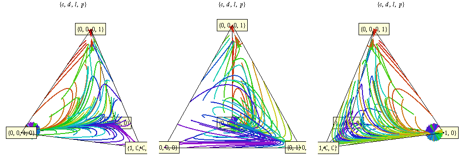
3D_trajectories

Note, that the result is not a vectorfield in 3D but a set of trajectories (of a 4D ODE on a 3D simplex). Accordingly, I look for solutions which comply to/deal with the following issues:

  1. Trajectories are specified as lists of points rather than individual vectors of a given position in space.
  2. A trajectory should be divisible to multiple arrows (streamlines), arranged neatly without any overlap.
  3. No streamlines should cross.
  4. A set of streamlines forming a trajectory should have its individual color.
  5. Arrows shouldn't start or end at the very same position.
  6. Interpolation of trajectories would be nice.

I have asked this question on Mathgroup (here and answers here), but as I haven't really dealt with the problem since (and did not develop it myself), it is still open. Heike already provided some useful stuff, but I think there is a lot of opportunity for improvement. (Heike, would you care to post your answers here as a solution please?)

Here is an updated toy example (posted without linebreaks not to flood page):

data = {{{0., 0., 1.}, {0.01, 0.01, 0.97}, {0.02, 0.02, 0.95}, {0.03, 0.02, 0.94}, {0.03, 0.02, 0.94}}, {{0., 0.17, 0.83}, {0.01, 0.08, 0.9}, {0.02, 0.04, 0.92}, {0.03, 0.03, 0.93}, {0.03, 0.02, 0.93}}, {{0., 0.33, 0.67}, {0.02, 0.17, 0.81}, {0.03, 0.09, 0.87}, {0.04, 0.05, 0.9}, {0.04, 0.03, 0.91}}, {{0., 0.5, 0.5}, {0.02, 0.28, 0.69}, {0.04, 0.15, 0.8}, {0.05, 0.08, 0.86}, {0.05, 0.05, 0.88}}, {{0., 0.67, 0.33}, {0.02, 0.43, 0.53}, {0.05, 0.26, 0.67}, {0.07, 0.16, 0.75}, {0.08, 0.11, 0.8}}, {{0., 0.83, 0.17}, {0.03, 0.64, 0.31}, {0.09, 0.48, 0.41}, {0.15, 0.4, 0.42}, {0.22, 0.39, 0.36}}, {{0.17, 0., 0.83}, {0.15, 0.01, 0.82}, {0.14, 0.02, 0.82}, {0.13, 0.03, 0.82}, {0.13, 0.04, 0.83}}, {{0.17, 0.17, 0.67}, {0.19, 0.16, 0.64}, {0.22, 0.16, 0.6}, {0.26, 0.19, 0.53}, {0.32, 0.25, 0.41}}, {{0.17, 0.33, 0.5}, {0.22, 0.33, 0.44}, {0.29, 0.38, 0.32}, {0.33, 0.48, 0.17}, {0.3, 0.63, 0.06}}, {{0.17, 0.5, 0.33}, {0.23, 0.52, 0.24}, {0.27, 0.6, 0.12}, {0.23, 0.71, 0.04}, {0.16, 0.81, 0.02}}, {{0.17, 0.67, 0.17}, {0.19, 0.71, 0.08}, {0.17, 0.79, 0.03}, {0.13, 0.85, 0.02}, {0.1, 0.88, 0.01}}, {{0.17, 0.83, 0.}, {0.09, 0.89, 0.01}, {0.07, 0.9, 0.01}, {0.07, 0.91, 0.01}, {0.07, 0.9, 0.01}}, {{0.33, 0., 0.67}, {0.37, 0.02, 0.59}, {0.45, 0.06, 0.48}, {0.53, 0.14, 0.31}, {0.56, 0.29, 0.13}}, {{0.33, 0.17, 0.5}, {0.39, 0.26, 0.34}, {0.42, 0.4, 0.17}, {0.35, 0.57, 0.06}, {0.24, 0.73, 0.02}}, {{0.33, 0.33, 0.33}, {0.36, 0.46, 0.17}, {0.31, 0.62, 0.06}, {0.21, 0.75, 0.02}, {0.14, 0.84, 0.01}}, {{0.33, 0.5, 0.17}, {0.29, 0.65, 0.06}, {0.2, 0.77, 0.02}, {0.13, 0.85, 0.01}, {0.09, 0.88, 0.01}}, {{0.33, 0.67, 0.}, {0.18, 0.81, 0.01}, {0.11, 0.87, 0.01}, {0.08, 0.9, 0.01}, {0.07, 0.9, 0.01}}, {{0.5, 0., 0.5}, {0.62, 0.03, 0.34}, {0.73, 0.1, 0.16}, {0.69, 0.23, 0.06}, {0.53, 0.44, 0.02}}, {{0.5, 0.17, 0.33}, {0.52, 0.32, 0.15}, {0.42, 0.52, 0.05}, {0.27, 0.70, 0.02}, {0.17, 0.81, 0.01}}, {{0.5, 0.33, 0.17}, {0.41, 0.53, 0.05}, {0.27, 0.70, 0.02}, {0.16, 0.82, 0.01}, {0.11, 0.87, 0.01}}};
Graphics3D[{Hue@RandomReal[], Arrow@#} & /@ data]
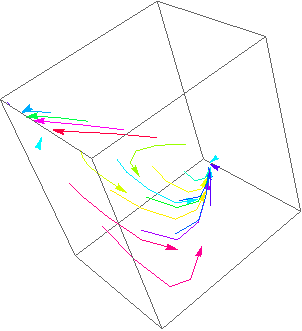
Mathematica graphics

$\endgroup$
11
  • 2
    $\begingroup$ The title of the question should be modified because this has nothing to so with stream lines, as the response to Eli's answer below indicates. Streamlines are defined by a vector field and a single starting point, not their start and end points. $\endgroup$
    – Jens
    Commented Feb 21, 2012 at 16:13
  • $\begingroup$ I wonder if you could define a gradient function on your trajectory to generate a vector field from your points to use in VectorPlot3D? $\endgroup$
    – Eli Lansey
    Commented Feb 21, 2012 at 16:26
  • $\begingroup$ @Jens, please suggest a better title. A streamline in my case is not only the start and endpoint, but is defined by a series of points. $\endgroup$ Commented Feb 21, 2012 at 16:41
  • $\begingroup$ @Eli: yes, that is something that could be done I guess. But it would be a different question (How to translate an n dimensional curve to an n dimensional vectorfield?). Also, VectorPlot3D would not be able to arrange arrows like StreamPlot does. $\endgroup$ Commented Feb 21, 2012 at 16:45
  • $\begingroup$ @IstvánZachar What about a 3D interpolation of the points, then ParametericPlot3D? It would help if you gave us some sample data. $\endgroup$
    – Eli Lansey
    Commented Feb 21, 2012 at 16:54

3 Answers 3

24
$\begingroup$

Let me add a few ideas, but be aware that this is unpolished code which was only hacked to show my points. I assume you have some kind of function $f(t;x_0,y_0,z_0)$ which gives you a trajectory starting at the initial point $(x_0,y_0,z_0)$ for $t=0$. I used $t$ only for convenience. Your function should be parametrized by the arc-lenc if you want a defined length for your field-lines

Let's consider some arbitrary pde I stole from the examples of NDSolve and create a function which takes an initial point, a length l, the number of points n and returns a StreamLine object containing n points of the trajectory

makeStreamLine[{x0_, y0_, z0_}, l_, n_] :=
 Block[{x, y, z},
  Block[{len = 
     Sqrt[(-3 (x[t] - y[t]))^2 + (-x[t] z[t] + 26.5 x[t] - 
          y[t])^2 + (x[t] y[t] - z[t])^2]},
   With[
    {sol = {x, y, z} /. First@NDSolve[{
          x'[t] == -3 (x[t] - y[t])/len,
          y'[t] == (-x[t] z[t] + 26.5 x[t] - y[t])/len,
          z'[t] == (x[t] y[t] - z[t])/len,
          x[0] == x0, z[0] == z0, y[0] == y0}, {x, y, z}, {t, 0, l}]
     },
    StreamLine[Table[Through[sol[t]], {t, 0, l, l/(n - 1.0)}]]
    ]
   ]
  ]

What you would maybe do in a first attempt is to take some random points from your domain of interest, use them as initial points, call the above function and get your StreamLines which you can draw as you like.

This is a bad idea for several reasons: First, the case where a random generator really creates nicely distributed seed points is really rare. Most of the times, the seed points are noticeably denser in some areas. But the real bad thing is, even if your seed points are nicely distributed, this does not mean that your stream-lines fill the space in a way it looks good.

The simple idea which solves this is to use a distance-transform. What you do is, you create exactly one StreamLine a a random place and then you calculate the next seed, by taking a point which is inside your domain, but as far as possible away from all already existing trajectory points.

The distance-transform is currently only available for images, so a very basic approach will help us out here. I sample the domain with Table, and use Nearest to calculate the seed with maximal distance. The function gets all previously calculated stream-lines, the domain and the number n of sampling points.

findNextSeedPoint[
  streamlines : {_StreamLine ..}, {{x0_, x1_}, {y0_, y1_}, {z0_, 
    z1_}}, n_] := 
 Block[{pts = Join @@ (streamlines /. StreamLine :> Sequence),
   nearestfunc, seed, maxDist = -1},
  nearestfunc = Nearest[pts];
  Table[With[{dist = Norm[{x, y, z} - First@nearestfunc[{x, y, z}]]},
    If[dist > maxDist,
     maxDist = dist;
     seed = {x, y, z}
     ]
    ],
   {z, z0, z1, (z1 - z0)/(n - 1.0)},
   {y, y0, y1, (y1 - y0)/(n - 1.0)},
   {x, x0, x1, (x1 - x0)/(n - 1.0)}];
  seed
  ]

What's left is the iteration of those two functions. The next function gets the domain, the length len of each stream-line, then number of stream-lines to create, the number of sampling points along each stream-line and the number of domain sampling points for the calculation of the next seed. As first initial point I use the center of the domain.

makeStreams[dim : {{x0_, x1_}, {y0_, y1_}, {z0_, z1_}}, len_, 
  nStreams_, nStreamPts_, regRes_] := Block[
  {seed = {x1 - x0, y1 - y0, z1 - z0}/2.0, streams},
  Nest[
   Append[#, 
     makeStreamLine[findNextSeedPoint[#, dim, regRes], len, 
      nStreamPts]] &, {makeStreamLine[seed, len, nStreamPts]}, 
   nStreams - 1]
  ]

Now you can plot the streams like you want. I use here the tubed 3d arrows

plotStreamLines[streams : {_StreamLine ..}] := 
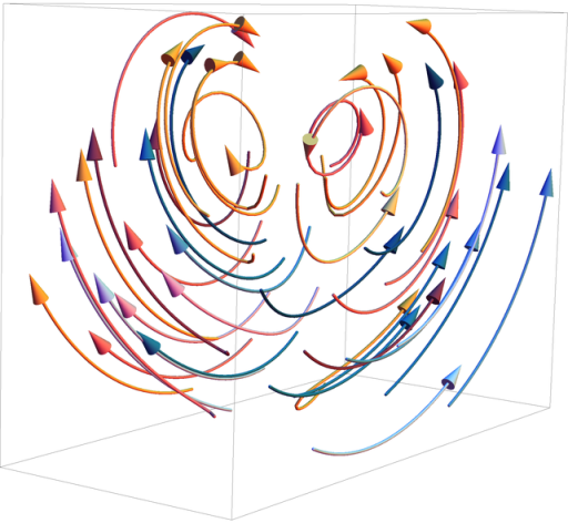
 Graphics3D[{ColorData[24, RandomInteger[{1, 12}]], 
     Arrow[Tube[#]]} & @@@ streams];

plotStreamLines@
 makeStreams[{{-20, 20}, {-20, 20}, {-20, 20}}, 50, 20, 57, 20]

enter image description here

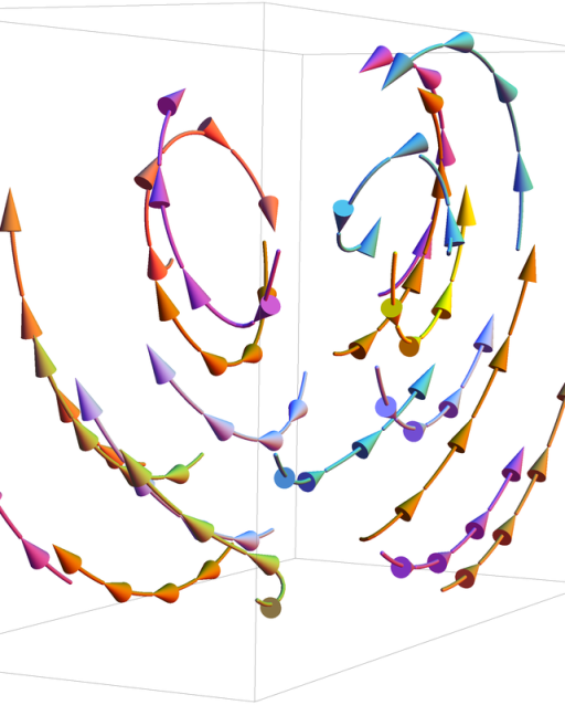
Heike showed in her post, how to create several arrows along one trajectory. This is of course possible too. A StreamLine object is only a series of points and you can surely partition this into several sublists where each one is displayed as its own arrow

enter image description here

There are several other extensions which could be implemented.

  • It is not ensured, that a stream-line does not leave the domain. What needs to be done is simply going through all stream-lines and using all points from the start until the domain is left. If all points are in, fine, if not, then you have some arrow, which are shorter.

  • While the seed points are nicely distributed, the stream-line itself can come really close to an already existing line. What could be useful is a function which cuts of stream-lines when they come too close to another one. With this you should get your domain filled without having the feeling, that there are too many arrows at some places

  • I just assumed, that you want field-lines with a defined length. You can of course integrate your lines as long as possible in both directions: You stop when they either leave the domain, reach a singularity or come too close together. If you look at the first example in the help of StreamPlot you notice exactly this behaviour.

$\endgroup$
1
  • $\begingroup$ nice post, StreamPlot also works via NDSolve. $\endgroup$
    – user21
    Commented Feb 22, 2012 at 8:49
14
$\begingroup$

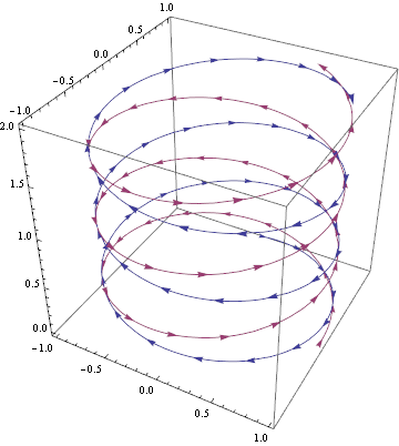
This is the same idea as in Heike's answer: replace the graphics primitives inside ParametricPlot3D:

 ParametricPlot3D[{{Sin[u], Cos[u], u/10}, {Cos[u], Sin[u], u/10}}, {u, 0, 20}] 
 /. Line[x_] :> Sequence[Arrowheads[Table[.025, {50}]], Arrow@Line[x]]

to get

parametric plot 3d with arrows

where the two numbers {0.025,50} control the sizes and the number of arrowheads.

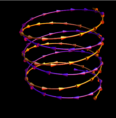
Update: Change the default value of Arrowheads using BaseStyle and post-process lines into tubes with arrows:

ParametricPlot3D[{{Sin[u], Cos[u], u/10}, {Cos[u], Sin[u], u/10}}, {u, 0, 20}, 
 PlotStyle -> (Directive[#, Specularity[White, 10]] & /@ {Purple,  Orange}),
 Boxed -> False, Axes -> False, Background -> GrayLevel[0], BoxRatios -> 1, 
 ImageSize -> 400,
 BaseStyle -> Arrowheads[Table[.05, {50}]]] /. Line -> Composition[Arrow, Tube[#, .015] &]

enter image description here


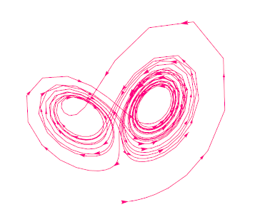
Another variation: For the solution to Lorenz equations

 trjctry =  NDSolve[{x'[t] == -3 (x[t] - y[t]), 
 y'[t] == -x[t] z[t] + 26.5 x[t] - y[t], z'[t] == x[t] y[t] - z[t], 
 x[0] == z[0] == 0, y[0] == 1}, {x, y, z}, {t, 0, 200},  MaxSteps -> Infinity]

partitioning the Line produced by ParametricPlot3D and taking every fifth segment in the partition:

 ParametricPlot3D[Evaluate[{x[t], y[t], z[t]} /. trjctry], {t, 0, 200},
 PlotPoints -> 50, BoxRatios -> {1, 1, 1}, Axes -> None, Boxed -> False] 
 /. (({a___, Line[xx_]} :> {a, Hue@RandomReal[], 
   Arrowheads[Table[#1, {#2}]], Arrow[Line[
     Partition[xx, Floor[Length[xx]/20]][[;; ;; 5]]]]}) & @@ {.02, 20})

we get

lorenz equations

$\endgroup$
9
$\begingroup$

These are the solutions I posted to mathgroup.

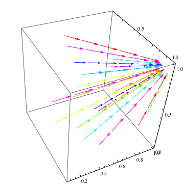
One way to mimic stream lines is to play around with Arrowheads. You can supply a list of positions along the curve at which to place an arrowhead, so you could do something like this:

startPts = RandomReal[{0, 1}, {20, 3}];
arrows = Arrow[{#, {1, 1, 1}}] & /@ startPts;
With[{narrows = 10}, 
 Graphics3D[{Arrowheads[Table[{0.02, i}, {i, 0, 1, 1/narrows}], 
    Appearance -> "Projected"], 
   Transpose[{Hue /@ RandomReal[1, 20], arrows}]}]]

Mathematica graphics

Note that this solution always places a fixed number arrows along the curve, independent of its length, so for short streamlines the arrow heads would be much closer together than for longer ones. Also, the streamlines are continuous curves whereas in StreamPlot you can choose to have gaps between the arrow segments.

Therefore, a different approach could be to parameterise the curves with respect to their arc length and plot each segment separately using for example ParametricPlot3D. For this approach we first need a function that produces an interpolation function of a list of coordinates:

Options[interpArcl] = Options[Interpolation];
interpArcl[plist_, opts : OptionsPattern[]] := 
 With[{arclengths = 
    Prepend[Accumulate[Norm /@ Differences[plist]], 0]},
  Interpolation[Transpose[{arclengths, plist}], opts]]

Next we need a function that will plot a sequence of arrows given a function f

Options[stream3D2] = Options[ParametricPlot3D];
stream3D2[f_, {min_, max_}, ds_, gap_, opts : OptionsPattern[]] :=
 Module[{segments, t},
  segments = 
   Table[Rescale[
     t, {0, 1}, {min + i ds, Min[min + (i + 1) ds - gap, max]}], {i, 
     0, Ceiling[(max - min)/ds] - 1}];
  ParametricPlot3D[Unevaluated[f /@ segments], {t, 0, 1}, {opts}] /. 
   a_Line :> Arrow[a]]

Here, {min, max} is the range for the arc length for which f should be plotted, ds is the length of each arrow segment, and gap is the gap between the segments.

Example:

startPts = RandomReal[{0, 1}, {20, 3}];
interplst = 
 interpArcl[{#, {1, 1, 1}}, InterpolationOrder -> 1] & /@ 
  startPts; 
plot = 
 Show[(MapIndexed[(stream3D2[#1, #1[[1, 1]], 0.2, 0.02, 
       RegionFunction -> 
        Function[{x, y, z}, 
         Sqrt[((x - 1)^2 + (y - 1)^2 + (z - 1)^2)] > 0.1], 
       PlotStyle -> 
        Directive[Hue[RandomReal[]], 
         Arrowheads[0.025, Appearance -> "Projected"]]]) &, 
    interplst]), PlotRange -> All]

Mathematica graphics

$\endgroup$

Your Answer

By clicking “Post Your Answer”, you agree to our terms of service and acknowledge you have read our privacy policy.

Not the answer you're looking for? Browse other questions tagged or ask your own question.