Poor convergence for first order PDE using FEM (Laplace's equation in a disk)

Question

Consider Laplace's eqn in the unit disk, r^2 D[u[r, t], {r, 2}] + r D[u[r, t], {r, 1}] + D[u[r, t], {t, 2}] == 0. The general analytic solution is easy to work out, and we can target the n=1 solution (i.e. u = r Cos[t]) using Dirichlet boundary conditions. The problem is easily solved with the finite element method:

uf1 = NDSolveValue[{r^2 D[u[r, t], {r, 2}] + r D[u[r, t], {r, 1}] + 
  D[u[r, t], {t, 2}] == 0, 
DirichletCondition[u[r, t] == Cos[t], r == 1 && t != 2 Pi], 
PeriodicBoundaryCondition[u[r, t], t == 2 \[Pi], 
 Function[x, x - {0, 2 \[Pi]}]]}, u, {r, 0, 1}, {t, 0, 2 Pi}];

Now let's try an alternative way to solve the same problem, using a first order PDE, D[u[r, t], r] == -I/r D[u[r, t], t], for a complex scalar field u. By separating u into its real and imaginary components, one can show that each satisfy the above Laplace's equation. We attempt to solve the PDE numerically, matching the Dirichlet condition above (for the real part):

uf2 = NDSolveValue[{D[u[r, t], r] == -I/r D[u[r, t], t], 
DirichletCondition[u[r, t] == Exp[I t], r == 1 && t != 2 Pi], 
PeriodicBoundaryCondition[u[r, t], t == 2 \[Pi], 
 Function[x, x - {0, 2 \[Pi]}]]}, u, {r, 0, 1}, {t, 0, 2 Pi}];

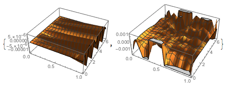
First things look OK: both solutions seem to approximate the exact target solution:

uA[r_, t_] = r Cos[t];
{Plot3D[Re[uf1[r, t]] - uA[r, t], {r, 0, 1}, {t, 0, 2 Pi}], Plot3D[Re[uf2[r, t]] - uA[r, t], {r, 0, 1}, {t, 0, 2 Pi}]}

but the conventional method is much better.

The question is: why does the 1st order method perform so poorly compared with the conventional (2nd order) method?

For the first order problem, Mathematica issues the usual warning about the equation being convection dominated, but can't we ignore this because we know the solutions are nice and smooth? (Btw, artificial diffusion doesn't help.) Is there an issue with applying FEM to first order PDEs, even if they are known to be elliptic?

A scan over MaxCellMeasure shows how serious the problem is:

errList1 = {}; errList2 = {};
For[n = 3, n <= 10, n++,
  mcm = 1./2^n;
  mesh = ToElementMesh[FullRegion[2], {{0, 1}, {0, 2 Pi}}, 
    MaxCellMeasure -> mcm];
  Quiet[
   uf1 = NDSolveValue[{r^2 D[u[r, t], {r, 2}] + r D[u[r, t], {r, 1}] +
         D[u[r, t], {t, 2}] == 0, 
      DirichletCondition[u[r, t] == Cos[t], r == 1 && t != 2 Pi], 
      PeriodicBoundaryCondition[u[r, t], t == 2 \[Pi], 
       Function[x, x - {0, 2 \[Pi]}]]}, u, {r, t} \[Element] mesh]; 
   uf2 = NDSolveValue[{D[u[r, t], r] == -I/r D[u[r, t], t], 
      DirichletCondition[u[r, t] == Exp[I t], r == 1 && t != 2 Pi], 
      PeriodicBoundaryCondition[u[r, t], t == 2 \[Pi], 
       Function[x, x - {0, 2 \[Pi]}]]}, u, {r, t} \[Element] mesh];
  ];
  err1 = Sqrt[
    Mean[Table[{ri, ti} = c; (Re[uf1[ri, ti]] - uA[ri, ti])^2, {c, 
       mesh["Coordinates"]}]]];
  err2 = Sqrt[
    Mean[Table[{ri, ti} = c; (Re[uf2[ri, ti]] - uA[ri, ti])^2, {c, 
       mesh["Coordinates"]}]]];
  AppendTo[errList1, {mcm, err1}];
  AppendTo[errList2, {mcm, err2}];
  ];
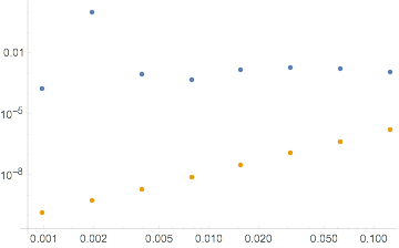
ListLogLogPlot[{errList2, errList1}]

Although the error of the first solution goes clearly as mcm^2, the error of the second solution does not even convincingly go to zero with mcm.

A final motivating comment: Although the above problem is easily evaded (though not understood) by using the usual second order formulation, one may be faced with a first order PDE that cannot be easily transformed into the standard 2nd order form. It would be useful to know how reliably solve an elliptic first order system.

Answer 1

I can offer a partial answer to this. There are two issues I found.

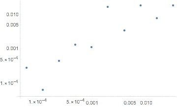
(1) The polar coordinates were problematic at high resolution (I suppose the coordinate singularity at the origin might have been causing a problem), which did not allow me to go to very small mesh measure. By changing to cartesian coordinates, I was able to push to very small resolution and get more convincing convergence with the first order PDE:

m = 3; uA[x_, y_] = (x + I y)^m;
errList = {};

For[n = 5, n <= 14, n++,
  mcm = 1./2^n;
  meshxy = ToElementMesh[Disk[], MaxCellMeasure -> mcm];
  Quiet[
   uf = NDSolveValue[{(x - I y) D[u[x, y], x] + (y + I x) D[u[x, y], 
           y] == 0, 
       DirichletCondition[u[x, y] == uA[x, y], x^2 + y^2 == 1]}, u, 
      Element[{x, y}, meshxy]];
   ];
  err = Sqrt[
    Mean[Table[{xi, yi} = c; (Norm[uf[xi, yi] - uA[xi, yi]])^2, {c, 
       meshxy["Coordinates"]}]]];
  AppendTo[errList, {mcm, err}];
  ];
ListLogLogPlot[errList]

The scaling of the error is only first order in the cell measure, but it is more convincing now.

(2) Poking around in FEM references, I noticed that first order PDEs have a reputation for being poorly handled by "standard" finite element methods, and some texts recommended a "least squares" approach (e.g. Ern, Guermond. Theory and Practice of Finite Elements (2004) chapter 5). This is equivalent to solving a related higher order PDE, but the format follows rather intuitively from the original PDE:

b = {x - I y, y + I x}; bs = {x + I y, y - I x};
PDE = -Div[bs b.Grad[u[x, y], {x, y}], {x, y}] == 0;

Now we do the error scan as before:

errList = {};
For[m = 5, m <= 14, m++, mcm = 1./2^m;
  meshxy = ToElementMesh[Disk[], MaxCellMeasure -> mcm];
  uf = NDSolveValue[{PDE, 
     DirichletCondition[u[x, y] == uA[x, y], x^2 + y^2 == 1]}, u, 
    Element[{x, y}, meshxy]];
  err = Sqrt[
    Mean[Table[{xi, yi} = c; (Norm[uf[xi, yi] - uA[xi, yi]])^2, {c, 
       meshxy["Coordinates"]}]]];
  AppendTo[errList, {mcm, err}];
  ];
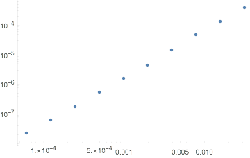
ListLogLogPlot[errList]

This error seems to scale as mcm^1.5.

EDIT

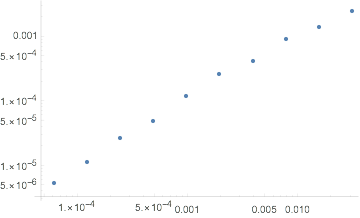
It may be possible to replicate the above performance, using FEM programming and post-processing, instead of solving the second order equation. Below is one idea that gives a slight improvement over the naive solution of the first order PDE (but does not do as well as solving the second order equation):

GetSystemMatricesLS[PDE_, iVars_, dVars_, mesh_] := Module[{nr, sd, vd, state, femdata, initBCs, initCoeffs, methodData, discretePDE, stiffness, load, LSstiffness, LSload, discreteBCs},
  nr = ToNumericalRegion[mesh];
  sd = NDSolve`SolutionData[{"Space" -> nr}]; 
  vd = NDSolve`VariableData[{"DependentVariables" -> dVars, 
     "Space" -> iVars}];
  methodData = InitializePDEMethodData[vd, sd];
  Quiet[{state} = 
    NDSolve`ProcessEquations[PDE, dVars, iVars \[Element] mesh, 
     Method -> {"FiniteElement"}]]; 
  femdata = state["FiniteElementData"];
  initBCs = femdata["BoundaryConditionData"];
  initCoeffs = femdata["PDECoefficientData"]; 
  discretePDE = DiscretizePDE[initCoeffs, methodData, sd];
  stiffness = discretePDE["StiffnessMatrix"]; 
  load = discretePDE["LoadVector"];
  discreteBCs = 
   DiscretizeBoundaryConditions[initBCs, methodData, sd];
  LSstiffness = ConjugateTranspose[stiffness].stiffness;
  LSload = ConjugateTranspose[stiffness].load;
  DeployBoundaryConditions[{LSload, LSstiffness}, discreteBCs];
  {LSstiffness, LSload}
  ]

Note how the transformation to a symmetrized stiffness matrix is performed before deploying the boundary conditions.

k = 3; uA[x_, y_] = (x + I y)^k;

errList = {};
For[n = 5, n <= 14, n++,
  mcm = 1./2^n;
  PrintTemporary["n: ", n];
  meshxy = ToElementMesh[Disk[], MaxCellMeasure -> mcm];
  {stiffness, load} = 
   GetSystemMatricesLS[{(x - I y) D[u[x, y], x] + (y + I x) D[u[x, y], 
         y] == 0, DirichletCondition[u[x, y] == uA[x, y], True]}, {x, 
     y}, {u}, meshxy];
  solution = LinearSolve[stiffness, load];
  uf = ElementMeshInterpolation[meshxy, solution];
  err = Sqrt[
    Mean[Table[{xi, yi} = c; (Norm[uf[xi, yi] - uA[xi, yi]])^2, {c, 
       meshxy["Coordinates"]}]]];
  AppendTo[errList, {mcm, err}];];
ListLogLogPlot[errList]