1
$\begingroup$

I have data of a function that goes like $f(x)\propto x ^\alpha $ for a certain range of $x$ and like $f(x)\propto x^\beta$ for another one. It is common in the literature to make a log log plot and then fit two straight lines in the corresponding regimes to show the different exponents. I was wondering how one can achieve this in Mathematica. Basically, the questions are

1) How to make a linear fit on loglog data?

2) How to make and show multiple linear fits on different ranges of the data?

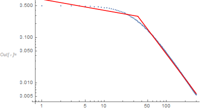
Answering to a comment that asked for more information: I don't have an analytical result for the crossover value $x_c$ at which the function changes regimes. Evenmore, it's not an inmediate change but there's a intermediate regime for values of $x$ close to the crossover where the function is not $f(x)\propto x ^\alpha $ or $f(x)\propto x^\beta$. Here I show a plot of the data in loglog scale.

enter image description here

The first regime is between 5 and 100 and the second one is in the last part of the data.

$\endgroup$
4
  • $\begingroup$ See mathematica.stackexchange.com/questions/192682/…? $\endgroup$
    – JimB
    Commented Oct 19, 2019 at 17:01
  • $\begingroup$ If you could give more information, it would be helpful. For example, do you know the value of $x$ that separates the two curves or does that value need to be estimated from the data? Can any of the data be made available? Do both parts have the same constant error variance in the log scale? $\endgroup$
    – JimB
    Commented Oct 19, 2019 at 19:51
  • $\begingroup$ Thanks for your comment! I'll edit with more information $\endgroup$ Commented Oct 19, 2019 at 20:59
  • $\begingroup$ could you please share a sample of your data? $\endgroup$
    – Fraccalo
    Commented Oct 20, 2019 at 8:47

2 Answers 2

1
$\begingroup$

Let's start by generating some sample data:

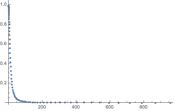
values = Table[{x, 100/(x^2 + 100)}, {x, PowerRange[1, 1000, 1.1]}];
ListPlot[values]

Mathematica graphics

On a log-log plot, it can be seen that this is the type of data that you have shown in your question:

ListLogLogPlot[values]

Mathematica graphics

It has two regimes; one behavior in the beginning, and one behavior at the end. We create two samples that represent these two regimes:

part1 = Select[values, First[#] < 2.5 &];
part2 = Select[values, First[#] > 100 &];
ListLogLogPlot[{part1, part2}]

Mathematica graphics

Now, we wish to find a linear fit for each of these two parts. In order to know what to do next, we need to understand ListLogLogPlot. What this function does is that it takes the Log of both the x and y values. It then changes the x-axis and y-axis tick labels, but it does not touch the underlying coordinate system. It is a purely cosmetic change. This means that, regardless of what the tick labels say, this is the coordinate system we're working with:

ListPlot[Log[values]]

Mathematica graphics

Consequently, all we need to do is this:

model1 = LinearModelFit[Log[part1], x, x];
model2 = LinearModelFit[Log[part2], x, x];

Show[
 ListLogLogPlot[values],
 Plot[{model1[x], model2[x]}, {x, 0, 7}, PlotStyle -> {Red, Green}]
 ]

Mathematica graphics

To reinforce my earlier point about the underlying coordinate system being exactly the same, I would also like to show you this plot:

Show[
 ListPlot[Log[values]],
 Plot[{model1[x], model2[x]}, {x, 0, 7}, PlotStyle -> {Red, Green}]
 ]

Mathematica graphics

$\endgroup$
0
$\begingroup$

If you only need to make predictions within Mathematica, then because of the low variability about the apparent smooth curve, you should use Interpolation. (It would be certainly more desirable if there was some theoretical curve function to consider.)

An alternative to interpolation, would be to use @AntonAntonov 's [Quantile regression]1.

But if you need a prediction equation to use outside of Mathematica and if two or more linear segments give what you would consider an adequate fit, then you should consider piecewise linear regression. Below is some code to estimate two linear segments along with estimating the break point.

(* Generate some data *)
data = Table[{x, 500/(x^2 + 1000)}, {x, 1, 300}];

(* Make sure that the two line segments join at the unknown cut point xc *)
sol = Solve[a1 + b1 xc == a2 + b2 xc, a2][[1]]
(* {a2 -> a1+b1 xc-b2 xc} *)

nlm = NonlinearModelFit[Log[data], 
   Boole[x <= xc] (a1 + b1 x) + Boole[x > xc] (a2 + b2 x) /. sol,
   {{a1, -0.5}, {b1, -0.13}, {b2, -2}, {xc, 3}}, x];
nlm["BestFitParameters"]
(* {a1 -> -0.36738734072224805, b1 -> -0.24323881420018847,
    b2 -> -1.8168252905594362, xc -> 3.5484803234032367} *)

Show[ListLogLogPlot[data],
 LogLogPlot[Exp[nlm[Log[x]]], {x, 1, 300}, PlotStyle -> Red]]

Data and fit

$\endgroup$

Your Answer

By clicking “Post Your Answer”, you agree to our terms of service and acknowledge you have read our privacy policy.

Not the answer you're looking for? Browse other questions tagged or ask your own question.