6
$\begingroup$

Background

I would like to numerically solve the stationary Stokes equation from fluid dynamics

$\eta_i \nabla^2 \vec{u}_i - \nabla p = 0$

with the incompressibility condition

$\nabla \cdot \vec{u} = 0$

for the flow field in two immiscible liquid layers with a spatially varying surface tension $\sigma(x)$ between them. In what follows I am assuming that the surface tension has a constant gradient: $\partial_x \sigma = 1$. This may be due to a temperature or concentration gradient at the interface, which does not get modelled explicitly for the sake of simplicity.

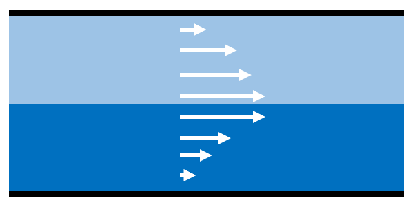
This should lead to waves that propagate transversal to the interface:

Marangoni_shear_flow

For more details, see e.g. Fig. 9.3a in https://ocw.mit.edu/courses/mathematics/18-357-interfacial-phenomena-fall-2010/lecture-notes/MIT18_357F10_Lecture9.pdf


Problem Outline

The spatial layout of the problem is depicted as follows: problem setup
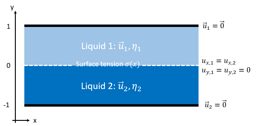
The integration domain is a two-dimensional box, which liquid 1 on top of liquid 2. Each have their respective viscosities $\eta_i$ and flow fields $\vec{u}_i$. At the top and bottom of the box are no-slip boundaries, which imply Dirichlet boundary conditions for the flow fields. At the interface the vertical components of each flow field are zero to enforce that both liquids can not mix. The flow tangential to the interface has the same magnitude due to continuity.

The surface tension at the interface adds another internal boundary condition that seems complicated at first sight:

$P_s \nabla \sigma = P_s (T_2-T_1) \vec{n}$.

Here $\vec{n}$ is the vector normal to the interface, $P_s$ projects a vector $\vec{v}$ on the interface (by removing its component normal to the interface) and the $T_i = \eta_i (\nabla\vec{u} + (\nabla\vec{u})^T)$ are strain-rate tensors. For the simple planar problem at hand, this allows us to reduce the surface tension condition to:

$\partial_x \sigma = \eta_2 \partial_y u_{x,2} - \eta_1 \partial_y u_{x,1}$

The analytical solution to this problem is:

$\vec{u}_i(x,y) = \frac{1 \pm y}{\eta_1+\eta_2}\partial_x \sigma \vec{e}_x$


Code

To verify this solution numerically, I wrote the following Mathematica code:

(** create mesh **)
boundaryMesh = ToBoundaryMesh[
   "Coordinates" -> {{0, -1}, {0, 0}, {0, 1}, {2, 1}, {2, 0}, {2, -1}},
   "BoundaryElements" -> {LineElement[{{1, 2}, {2, 3}, {3, 4}, {4, 
        5}, {5, 6}, {6, 1}, {2, 5}}]}
   ];
p1 = boundaryMesh["Wireframe"];
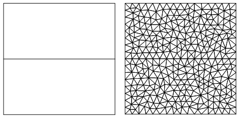
mesh = ToElementMesh[boundaryMesh, MaxCellMeasure -> 0.01];
p2 = mesh["Wireframe"];
Grid[{{p1, p2}}]

This gives me the following mesh with the required internal boundary:

meshes

The PDE and boundary conditions are defined as follows. Note that I am not defining separate flow fields for the top and bottom, but instead I tried to throw everything into one flow field with hoizontal and vertical components u, v.

\[Eta]=With[{\[Eta]1=0.5,\[Eta]2=1},If[y<0,\[Eta]1,\[Eta]2]];

(** u,v,p = horizontal speed, vertical speed, pressure **)
pde={
 Inactive[Div][\[Eta] Inactive[Grad][u[x, y], {x, y}], {x, y}] + (p^(1,0))[x, y]==0,
 Inactive[Div][\[Eta] Inactive[Grad][v[x, y], {x, y}], {x, y}] + (p^(0,1))[x, y]==0,
 (u^(1,0))[x, y]+(v^(0,1))[x, y]==0
};

boundaryConditions = {
   DirichletCondition[{u[x, y] == 0, v[x, y] == 0, p[x, y] == 0}, (y == -1 \[Or] y == 1) \[And] (0 < x < 2)],
   DirichletCondition[v[x, y] == 0, y == 0]
   }; 

(** solve flow velocities with a method that is an order higher than pressure for stable solutions **)
{xVel, yVel, pressure} = NDSolveValue[
   {pde, boundaryConditions},
   {u, v, p},
   {x, y} \[Element] mesh,
   Method -> {"FiniteElement", 
     "InterpolationOrder" -> {u -> 2, v -> 2, p -> 1}}
];

plot=VectorPlot[{xVel[x, y], yVel[x, y]}, {x, y} \[Element] mesh, 
 AspectRatio -> Automatic, StreamPoints -> 6, 
 StreamColorFunction -> "TemperatureMap", 
 StreamColorFunctionScaling -> False]

The obviously unsatisfying result is:

result


Questions

  1. The solution to my code is pretty boring (no flow), because I did not include the internal boundary condition for the surface tension:

$\partial_x \sigma = \eta_2 \partial_y u_{x,2} - \eta_1 \partial_y u_{x,1}$

with

$\partial_x \sigma = 1$.

How can I do that? It is not clear to me how to enforce an internal jump in the derivative by a prescribed amount using NeumannValue[]. Do I need to run 2 NDSolve's for each region in tandem as described here: FEM-ception: Using output of NDSolve FEM as input in another FEM problem ? And then have the solution in one domain as a boundary condition for the simulation in the other? Also note that this is more complicated than a simple jump in a spatially-dependent parameter, as solved here: Neumann boundary condition on a boundary inside the region. This problem involves a jump in a derivative by a specified amount.

  1. How can I set periodic boundary conditions? I tried PeriodicBoundaryCondition[u[x, y], x == 0, TranslationTransform[{2, 0}]],PeriodicBoundaryCondition[v[x, y], x == 0, TranslationTransform[{2, 0}]] but then I got this error: NDSolveValue::femnodpbc: DirichletCondition can not be present on the target boundary of a PeriodicBoundaryConditon.

This problem is a first test for me of Mathematica's FEM capabilities, I later intend to apply the discontinuous surface tension boundary condition to a sphere geometry in 3D.

$\endgroup$
5
  • 1
    $\begingroup$ In this problem, a moving boundary must be introduced. $\endgroup$ Commented Oct 14, 2019 at 13:55
  • $\begingroup$ Could you elaborate more on the "moving boundary"? In the outlined problem I want all boundaries to be fixed in space. This is the case when Marangoni convection leads to transverse surface waves (low Prandtl number) and not to the convection rolls that lead to a wavy interface (large Prandtl number). See e.g. Fig. 9.3a in ocw.mit.edu/courses/mathematics/… $\endgroup$
    – Oscillon
    Commented Oct 14, 2019 at 17:32
  • $\begingroup$ "Marangoni flows may be generated by gradients in either temperature or chemical composition at an interface". You have no temperature or concentration in the model. Your model has a different viscosity and different velocity (and density?) set at the interface. $\endgroup$ Commented Oct 14, 2019 at 18:03
  • $\begingroup$ I see that I should have formulated the problem clearer. At the interface I defined a spatially-dependent surface tension $\sigma$, with a constant spatial gradient. This causes a flow, called Marangoni flow. In this simple case, I am not modelling what causes the surface tension gradient (temperature/concentration gradients). I'll edit the question to make this clearer. $\endgroup$
    – Oscillon
    Commented Oct 14, 2019 at 18:29
  • $\begingroup$ @Oscillon I am also interested in establishing a surface tension gradient over a Disk or a sphere to model deformation in a biological context. It would be great if we can talk :) please let me know. thanks ! $\endgroup$
    – Ali Hashmi
    Commented Aug 3, 2020 at 15:26

1 Answer 1

3
$\begingroup$

This code reproduces the analytical solution with high accuracy.

<< NDSolve`FEM`
H = 1; L = 2; \[CapitalOmega]1 = 
 Rectangle[{0, 0}, {L, H}]; \[CapitalOmega]2 = 
 Rectangle[{0, -H}, {L, 0}];
RegionPlot[RegionUnion[\[CapitalOmega]1, \[CapitalOmega]2], 
 AspectRatio -> Automatic]
mesh1 = ToElementMesh[\[CapitalOmega]1, 
  "MaxCellMeasure" -> 0.001]; mesh2 = 
 ToElementMesh[\[CapitalOmega]2, "MaxCellMeasure" -> 0.001];

k = 5; t0 = 1/10; sx = 1; mu1 = 1/2; mu2 = 1;
U0[y_, t_] := sx (1 - y)/(mu1 + mu2);
U1[0][x_, y_] := sx (1 - y)/(mu1 + mu2);
V1[0][x_, y_] := 0;
P1[0][x_, y_] := 0; U2[0][x_, y_] := sx (1 + y)/(mu1 + mu2);
V2[0][x_, y_] := 0;
P2[0][x_, y_] := 0;
S[0][x_] := 0;
Do[
  {U1[i], V1[i], P1[i]} = 
   NDSolveValue[{{Inactive[
           Div][({{-\[Mu], 0}, {0, -\[Mu]}}.Inactive[Grad][
             u[x, y], {x, y}]), {x, y}] + 
\!\(\*SuperscriptBox[\(p\), 
TagBox[
RowBox[{"(", 
RowBox[{"1", ",", "0"}], ")"}],
Derivative],
MultilineFunction->None]\)[x, y] + (u[x, y] - U1[i - 1][x, y])/t0 + 
         U1[i - 1][x, y]*D[u[x, y], x] + 
         V1[i - 1][x, y]*D[u[x, y], y], 
        Inactive[
           Div][({{-\[Mu], 0}, {0, -\[Mu]}}.Inactive[Grad][
             v[x, y], {x, y}]), {x, y}] + 
\!\(\*SuperscriptBox[\(p\), 
TagBox[
RowBox[{"(", 
RowBox[{"0", ",", "1"}], ")"}],
Derivative],
MultilineFunction->None]\)[x, y] + (v[x, y] - V1[i - 1][x, y])/t0 + 
         U1[i - 1][x, y]*D[v[x, y], x] + 
         V1[i - 1][x, y]*D[v[x, y], y], 
\!\(\*SuperscriptBox[\(u\), 
TagBox[
RowBox[{"(", 
RowBox[{"1", ",", "0"}], ")"}],
Derivative],
MultilineFunction->None]\)[x, y] + 
\!\(\*SuperscriptBox[\(v\), 
TagBox[
RowBox[{"(", 
RowBox[{"0", ",", "1"}], ")"}],
Derivative],
MultilineFunction->None]\)[x, y]} == {NeumannValue[1/2, y == 0], 0, 
        0} /. \[Mu] -> mu1, {
      DirichletCondition[{u[x, y] == U0[y, i*t0], v[x, y] == 0}, 
       x == 0.], 
      DirichletCondition[{u[x, y] == 0., v[x, y] == 0.}, 
       0 <= x <= L && y == H], 
      DirichletCondition[p[x, y] == P1[i - 1][x, y], x == L], 
      DirichletCondition[{u[x, 
          y] == (U1[i - 1][x, y] + U2[i - 1][x, y])/2, v[x, y] == 0}, 
       y == 0]}}, {u, v, p}, {x, y} \[Element] mesh1, 
    Method -> {"FiniteElement", 
      "InterpolationOrder" -> {u -> 2, v -> 2, p -> 1}}]; {U2[i], 
    V2[i], P2[i]} = 
   NDSolveValue[{{Inactive[
           Div][({{-\[Mu], 0}, {0, -\[Mu]}}.Inactive[Grad][
             u[x, y], {x, y}]), {x, y}] + 
\!\(\*SuperscriptBox[\(p\), 
TagBox[
RowBox[{"(", 
RowBox[{"1", ",", "0"}], ")"}],
Derivative],
MultilineFunction->None]\)[x, y] + (u[x, y] - U2[i - 1][x, y])/t0 + 
         U2[i - 1][x, y]*D[u[x, y], x] + 
         V2[i - 1][x, y]*D[u[x, y], y], 
        Inactive[
           Div][({{-\[Mu], 0}, {0, -\[Mu]}}.Inactive[Grad][
             v[x, y], {x, y}]), {x, y}] + 
\!\(\*SuperscriptBox[\(p\), 
TagBox[
RowBox[{"(", 
RowBox[{"0", ",", "1"}], ")"}],
Derivative],
MultilineFunction->None]\)[x, y] + (v[x, y] - V2[i - 1][x, y])/t0 + 
         U2[i - 1][x, y]*D[v[x, y], x] + 
         V2[i - 1][x, y]*D[v[x, y], y], 
\!\(\*SuperscriptBox[\(u\), 
TagBox[
RowBox[{"(", 
RowBox[{"1", ",", "0"}], ")"}],
Derivative],
MultilineFunction->None]\)[x, y] + 
\!\(\*SuperscriptBox[\(v\), 
TagBox[
RowBox[{"(", 
RowBox[{"0", ",", "1"}], ")"}],
Derivative],
MultilineFunction->None]\)[x, y]} == {NeumannValue[1/2, y == 0], 0, 
        0} /. \[Mu] -> mu2, {
      DirichletCondition[{u[x, y] == U0[-y, i*t0], v[x, y] == 0}, 
       x == 0.], 
      DirichletCondition[{u[x, y] == 0., v[x, y] == 0.}, 
       0 <= x <= L && y == -H], 
      DirichletCondition[p[x, y] == P2[i - 1][x, y], x == L], 
      DirichletCondition[{u[x, 
          y] == (U1[i - 1][x, y] + U2[i - 1][x, y])/2, v[x, y] == 0}, 
       y == 0]}}, {u, v, p}, {x, y} \[Element] mesh2, 
    Method -> {"FiniteElement", 
      "InterpolationOrder" -> {u -> 2, v -> 2, p -> 1}}]; 
  S[i] = mu2 Derivative[0, 1][U2[i]][x, 0] - 
    mu1 Derivative[0, 1][U1[i]][x, 0], {i, 1, k}];

Streamlines

{StreamDensityPlot[{U1[k][x, y], 
   V1[k][x, y]}, {x, y} \[Element] \[CapitalOmega]1, 
  StreamStyle -> LightGray, ColorFunction -> "Rainbow", 
  PlotLegends -> Automatic, AspectRatio -> Automatic], 
 StreamDensityPlot[{U2[k][x, y], 
   V2[k][x, y]}, {x, y} \[Element] \[CapitalOmega]2, 
  StreamStyle -> LightGray, ColorFunction -> "Rainbow", 
  PlotLegends -> Automatic, AspectRatio -> Automatic]}

Figure 1

Inlet and outlet velocity profile and accuracy of boundary conditions $v_1(x,0)=v_2(x,0)=0$

Plot[{U1[k][L, y], U2[k][L, y], U1[k][0, y], U2[k][0, y]}, {y, -H, H},
  AspectRatio -> Automatic]

Plot[{V1[k][x, 0], V2[k][x, 0]}, {x, 0, L}, PlotRange -> All]

Figure 2

$\endgroup$
5
  • $\begingroup$ I see that you tackle the problem by solving the equations separately in each domain. Does this mean that Mathematica does not support internal jump boundaries for derivatives? $\endgroup$
    – Oscillon
    Commented Oct 15, 2019 at 3:19
  • $\begingroup$ Going through your code, I have a number of questions: 1) What is U[i] - it's not an array, right? What is the advantage of using U[i] over U[[i]]? 2) What are t0 and sx? 3) What is this the reasoning for this term: + (u[x, y] - U1[i - 1][x, y])/t0 ? 4) Did you include an additional convective term: + U1[i - 1][x, y]*D[u[x, y], x] + V1[i - 1][x, y]*D[u[x, y], y]? Did you include it, because it stabilizes the solution? $\endgroup$
    – Oscillon
    Commented Oct 15, 2019 at 3:29
  • $\begingroup$ 5) At the interface you set the horizontal flow to the average DirichletCondition[{u[x, y] == (U1[i - 1][x, y] + U2[i - 1][x, y])/2, v[x, y] == 0}, y == 0] instead of the value from the respective other flow field. Why is that? 6) The surface tension gradient gets calculated, but is not used in the Neumann boundary condition. Shouldn't it be (mu2 Derivative[0, 1][U2[i]][x, 0] - nablaS)/mu1 for U1? $\endgroup$
    – Oscillon
    Commented Oct 15, 2019 at 3:35
  • $\begingroup$ 7) Is it faster to use {{-\[Mu], 0}, {0, -\[Mu]}}.Inactive[Grad] than -\[Mu].Inactive[Grad]? $\endgroup$
    – Oscillon
    Commented Oct 15, 2019 at 3:47
  • $\begingroup$ Here we solve the system of Navier-Stokes equations for an incompressible flow -see community.wolfram.com/groups/-/m/t/1433064 $\endgroup$ Commented Oct 15, 2019 at 10:31

Your Answer

By clicking “Post Your Answer”, you agree to our terms of service and acknowledge you have read our privacy policy.

Not the answer you're looking for? Browse other questions tagged or ask your own question.