Adaptive Meshrefinement NDSolve&FiniteElements

Question

In a simple example I try to solve the heat equation using NDSolve and Method->"FiniteElement". I know that NDSolve gives the solution as an interpolationfunction inside an ElementMesh.

First the mesh is created

Needs["NDSolve`FEM`"]
disc = ImplicitRegion[  x^2 + y^2 <= 1 && 0 <= z <= 1/10, {x, y , z}];
mesh = DiscretizeRegion[disc, MaxCellMeasure -> {"Volume" -> Pi/10}];
MeshCells[mesh, 3] // Length  (*36279*)

The mesh has around 36000 elements.

Simulation inside this mesh

U = NDSolveValue[{ 0 ==    Laplacian[u[ x, y, z ] , {x, y, z }]+ 50NeumannValue[1,  x >= 0 && y >= 0 && z == 1/10     ]-  1     NeumannValue[u[ x, y, z] - 20, z == 1/10] },u, 
Element[{x, y, z }, mesh ] , Method -> "FiniteElement"] 
DensityPlot[U[x, y, 1/10],Element[{x, y}, ImplicitRegion[x^2 + y^2 <= 1, {x, y}]],ColorFunction -> (ColorData["TemperatureMap"][#1] &),MaxRecursion -> 4]

gives a feasible solution

with considerably refined mesh

U["ElementMesh"]
(*TetrahedronElement["<" 160748 ">"]*) 

consisting of now 160748 elements, that means 440% increase of meshsize!

My question: Is it possible to keep the initial mesh mesh unchanged(fixed) by NDSolve?

Thanks!

Answer 1

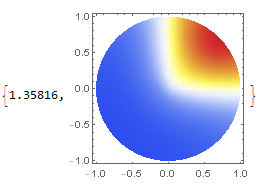
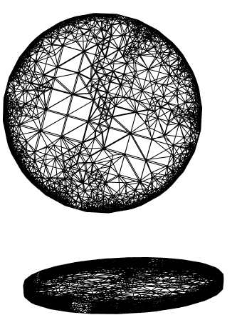
If you use ToElementMesh versus DiscretizeRegion and look at the "Wireframe", then you will see that your mesh looks pretty ugly.

mesh["Wireframe"]

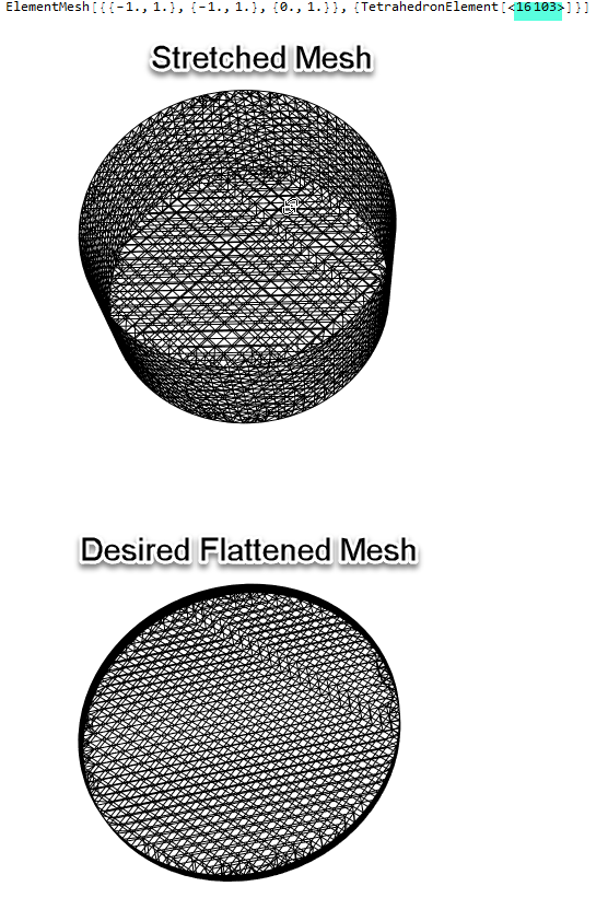
You can make a prettier mesh by starting with a geometry that has more cube-like aspect ratio and then scale the z-coordinate and remesh as shown below:

Needs["NDSolve`FEM`"]
(* Stretch Disc Region for better aspect ratio *)
disc = ImplicitRegion[x^2 + y^2 <= 1 && 0 <= z <= 1, {x, y, z}];
mesh0 = ToElementMesh[disc]
mesh0["Wireframe"]
(* Scale z-coords and create new ElementMesh *)
crd = mesh0["Coordinates"];
crd[[All, 3]] = crd[[All, 3]]/10;
mesh = ToElementMesh["Coordinates" -> crd, 
   "MeshElements" -> mesh0["MeshElements"], 
   "BoundaryElements" -> mesh0["BoundaryElements"], 
   "PointElements" -> mesh0["PointElements"]];
mesh["Wireframe"]

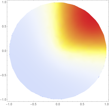
Now, you can perform your NDSolveValue in the following way and it should default to the FEM method.

U = NDSolveValue[{-Laplacian[
      u[x, y, z], {x, y, z}] == +50 NeumannValue[1, 
       x >= 0 && y >= 0 && z == 1/10] - 
     1 NeumannValue[u[x, y, z] - 20, z == 1/10]}, u, 
  Element[{x, y, z}, mesh]]
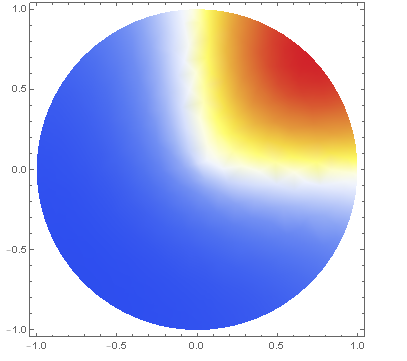
DensityPlot[U[x, y, 1/10], 
 Element[{x, y}, ImplicitRegion[x^2 + y^2 <= 1, {x, y}]], 
 ColorFunction -> (ColorData["TemperatureMap"][#1] &)]

Now, you can verify that the solution required about 10x fewer elements than the original approach.

U["ElementMesh"]
(* ElementMesh[{{-1., 1.}, {-1., 1.}, {0., 
   0.1}}, {TetrahedronElement["<" 16103 ">"]}] *)

Speed Improvement

In 3D problems, it is often useful to extract boundary meshes for visualizations. Below, I show a method to extract the top surface for the DensityPlot. The overhead in extracting the top surface is dwarfed by the efficiency gains in the DensityPlot function. On my machine, the following code was 350x faster than the code in the OP an 16.7x faster than the code above.

AbsoluteTiming[
 (* Stretch Disc Region for better aspect ratio *)
 disc = ImplicitRegion[x^2 + y^2 <= 1 && 0 <= z <= 1, {x, y, z}];
 mesh0 = ToElementMesh[disc];
 (* Scale z-coords and create new ElementMesh *)
 crd = mesh0["Coordinates"];
 crd[[All, 3]] = crd[[All, 3]]/10;
 mesh = ToElementMesh["Coordinates" -> crd, 
   "MeshElements" -> mesh0["MeshElements"], 
   "BoundaryElements" -> mesh0["BoundaryElements"], 
   "PointElements" -> mesh0["PointElements"]];
 U = NDSolveValue[{-Laplacian[
       u[x, y, z], {x, y, z}] == +50 NeumannValue[1, 
        x >= 0 && y >= 0 && z == 1/10] - 
      1 NeumannValue[u[x, y, z] - 20, z == 1/10]}, u, 
   Element[{x, y, z}, mesh]];
 (* Extract Top Surface as 2D Mesh *)
 (* Select Top Surface by Normal *)
 mask = (0.9999 < -{0, 0, 1}.#) & /@ mesh0["BoundaryNormals"][[1]];
 topelmi = 
  Pick[ElementIncidents[mesh0["BoundaryElements"]][[1]], mask];
 (* Extract unique incidents from top surface *)
 unique = DeleteDuplicates@Flatten[topelmi];
 (* Create an associate to renumber connectivity *)
 crddict = AssociationThread[unique -> Range@Length@unique];
 crd2d = mesh0["Coordinates"][[All, 1 ;; 2]];
 crd2dtop = crd2d[[unique]];
 newincidents = MapAt[crddict, topelmi, {All, All}];
 mesh2d = 
  ToElementMesh["Coordinates" -> crd2dtop, 
   "MeshElements" -> {TriangleElement[newincidents]}];
 (* Plot using new 2D mesh *)
 DensityPlot[U[x, y, 1/10], {x, y} \[Element] mesh2d, 
  ColorFunction -> (ColorData["TemperatureMap"][#1] &)]
 ]