Generate coefficient array from general formula of linear equation system

Question

This is a problem coming out in the implementation of finite difference method (FDM).

Here is a toy example. Suppose we want to solve the boundary value problem (BVP)

$$y''(x)=\sin(x),\ y(0)=0,\ y(1)=0$$

eq = y''[x] == Sin[x];
bc = {y[0] == 0, y[1] == 0};

with FDM, then we can program as follows. First, write down the corresponding difference formula:

Clear@dx;
generalformula = (y[x + dx] - 2 y[x] + y[x - dx])/dx^2 == Sin[x];

Then define the grid size and generate difference equations at every grid point:

points = 25; domain = {0, 1};
dx = Subtract @@ domain/(1 - points);
var = Table[y[x], {x, ##, dx}] & @@ domain;
differenceeq = Table[generalformula, {x, domain[[1]] + dx, domain[[-1]] - dx, dx}]~Join~bc;

Finally solve the difference equations with e.g. NSolve:

solrule = NSolve[differenceeq, var][[1]]; // AbsoluteTiming
(* {0.00462427, Null} *)

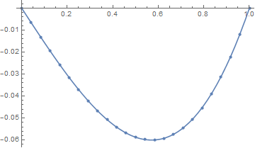
BTW, a comparision with the analytic solution:

asol = DSolveValue[{eq, bc}, y, x]
Plot[asol[x], {x, ##}, PlotRange -> All]~Show~
   ListPlot[solrule[[All, -1]], DataRange -> {##}] & @@ domain

Alternatively, we can extract the coefficient array from differenceeq and solve it with LinearSolve, as illustrated in the document of CoefficientArrays. This approach is faster than the one using NSolve:

{barray, marray} = CoefficientArrays[differenceeq, var]; // AbsoluteTiming
(* {0.000614324, Null} *)
sol = LinearSolve[marray // N, -barray]; // AbsoluteTiming
(* {0.000488251, Null} *)

However, this isn't the end. As already mentioned, we've generated difference equation at every grid point and then extract the coefficient array from the symbolic system in the code above. This procedure can be rather memory-demanding and slow when points is large. Is it possible to generate barray and marray directly from generalformula and bc programatically, in a memory-conserving and not-that-slow way?

---

If the toy example above is too simple to illustrate the underlying problem, the following is a more complicated one attempting to solve the problem mentioned here:

r = .8; glass = (1.45)^2; air = 1.; k = (2 π)/1.55;
n2 = Function[{x, y}, #] &@If[x^2 + y^2 <= r^2, glass, air];
ClearAll[fw, bw, delta]
SetAttributes[#, HoldAll] & /@ {fw, bw};

fw@D[expr_, x_] := 
 With[{Δ = delta@ToString@x}, 
  Subtract @@ (expr /. {{x -> x + Δ}, {x -> x}})/Δ]
bw@D[expr_, x_] := 
 With[{Δ = delta@ToString@x}, 
  Subtract @@ (expr /. {{x -> x}, {x -> x - Δ}})/Δ]

delta[a_ + b_] := delta@a + delta@b
delta[k_. delta[_]] := 0
grad = Function[expr, fw@D[expr, #] & /@ {x, y}];
div = Function[expr, Total@MapThread[bw@D@## &, {expr, {x, y}}]];
elst = e[#][x, y] & /@ Range[2];
discretelhs = 
  With[{n2 = n2[x, y]}, 
   div@grad@elst + (n2 k^2) elst - grad[div@elst - 1/n2 div[n2 elst]]] // FullSimplify;
points = 100; L = 2; domain = {-L, L}; grid = Array[# &, points, domain];
del = #[[2 ;; -2]] &;
delta["x"] = delta["y"] = -Subtract @@ domain/(points - 1);
vare = Outer[e[#][#2, #3] &, Range@2, del@grid, del@grid, 1] // Flatten;
discretelhslst = 
   Flatten@Transpose[
     Table[discretelhs, {x, del@grid}, {y, del@grid}], {2, 3, 1}]; // AbsoluteTiming
{barray2, marray2} = CoefficientArrays[discretelhslst, vare]; // AbsoluteTiming
{val, vec} = 
   Eigensystem[marray2, -6, 
    Method -> {"Arnoldi", "Shift" -> k^2 glass}]; // AbsoluteTiming
mat = ArrayReshape[#, {2, points - 2, points - 2}] & /@ vec;
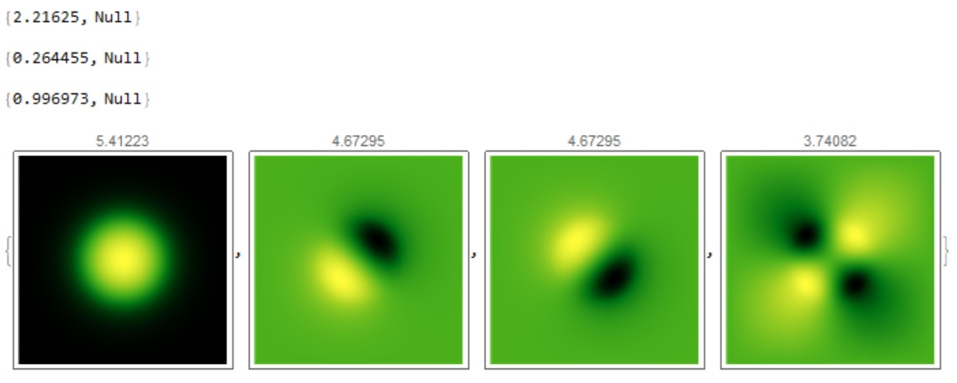
MapThread[ArrayPlot[#[[1]], PlotLabel -> Sqrt@#2, PlotRange -> All, 
   ColorFunction -> "AvocadoColors"] &, {mat, val}]

ByteCount[marray2]/1024^2. "MB"
(* 1.60567 "MB" *)

ByteCount[discretelhslst]/1024^2. "MB"
(* 44.9877 "MB" *)

The corresponding problem is, how to arrive at marray2 from discretelhs without generating discretelhslst, in an efficient enough way?

Answer 1

Partial ND

It's possible to again extract all this weight data and stuff in the higher dimensional cases using effectively the same procedure as for the 1D:

fdmWeightDataND~SetAttributes~HoldAll;
fdmWeightDataND[a_, dep_Symbol, indeps : {__Symbol}, hs : {__Symbol}] :=

  Block[{dep}, Block[indeps, Block[hs,
     Module[{weights, order, denomWeight, denom, num, powed, pows, minpow, 
       pts, x}, denom = Denominator[a];
      (*assumes the mesh spacing is in there at different powers*)

      order = Exponent[denom, #] & /@ hs;
      (*pull the power on the mesh spacing*)

      denomWeight = If[order > 0, Coefficient[denom, hs^order], denom];
      num = Numerator[a];
      {powed, pows} =
       Reap[
        num /.
         dep[args___]?(Not@*FreeQ[Alternatives @@ indeps]) :>
          dep @@
           Sow[
            MapThread[
             Coefficient[#, #2] &,
             {
              {args},
              hs
              }
             ]
            ]
        ];
      minpow = Min[pows];
      weights =
       AssociationThread[
        pows[[1]],
        Map[Coefficient[powed /. (dep @@ #) -> x, x] &, pows[[1]]]
        ];
      <|
       "Weights" -> weights,
       "Orders" -> order
       |>
      ]
     ]
    ]
   ];

This is less automate-able, though, since you need to specify what your f, independent variables, and mesh spacings are. Also without knowing how you'd like to flatten your nD tensor of grid points it's impossible to automatically build the FD matrix. But at a minimum I can give you weights and indices for the weights:

(*didn't want to Wikipedia the nine-point stencil so most of this is fake*)

simpleFormula = (
    f[x - xh, y] + f[x + xh, y] +
     f[x, y - yh] + f[x, y + yh] - 4 f[x, y] +
     1/2 f[x + xh, y - yh] + 1/2 f[x - xh, y - yh] +
     1/2 f[x + xh, y + yh] + 1/2 f[x - xh, y + yh]
    )/(xh^2*yh^2);

weights2D = fdmWeightDataND[simpleFormula, f, {x, y}, {xh, yh}]

<|"Weights" -> <|{0, 0} -> -4, {0, -1} -> 1, {0, 1} -> 1, {-1, 0} -> 
    1, {-1, -1} -> 1/2, {-1, 1} -> 1/2, {1, 0} -> 1, {1, -1} -> 1/2, {1, 1} ->
     1/2|>, "Orders" -> {2, 2}|>

Basically now you'd pick how to order your grid points and build a matrix from that. Here's one way to do this based on having the second index be the slowest moving (note that I'm only like 50% confident I built this correctly):

FDM2D[weightData_, {hx_, hy_}, {nptsx_, nptsy_}] :=

 Module[{xps, yps, weights = weightData["Weights"], 
   orders = weightData["Orders"]},
  xps = Length@DeleteDuplicates@Keys[weights][[All, 1]];
  yps = Length@Sort@DeleteDuplicates@ Keys[weights][[All, 2]];
  SparseArray[
    Flatten@
     KeyValueMap[
      With[{ix = #[[1]], iy = #[[2]], v = #2},
        Map[
         Band[
            If[ix >= 0, {1, 1 + ix}, {1 - ix, 1}] + {#, #} +
             If[iy >= 0, {0, iy*nptsx}, {-iy*nptsx, 0}],
            {nptsx*nptsy, nptsx*nptsx},
            {nptsx, nptsx}
            ] -> v &,
         Range[nptsx - Abs[ix]] - 1
         ]
        ] &,
      weights
      ],
    {nptsx*nptsy, nptsx*nptsx}
    ]/(Times @@ ({hx, hy}^orders))
  ]

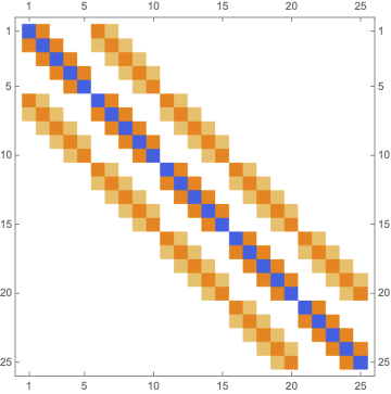
Here's what that outputs:

FDM2D[weights2D, {1, 1}, {5, 5}] // MatrixPlot

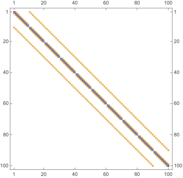
In the case of no coupling across degrees of freedom this looks correct I believe... (but can't be sure since I usually do my Laplacian via a Kronecker sum):

laplacian = (
    f[x - xh, y] + f[x + xh, y] +
     f[x, y - yh] + f[x, y + yh] - 4 f[x, y]
    )/(xh^2*yh^2);

FDM2D[fdmWeightDataND[laplacian, f, {x, y}, {xh, yh}], {1, 1}, {10, 
   10}] // MatrixPlot

Full Thing for 1D

Here's a method that automates this extraction for 1D FDM stuff:

fdmWeightData~SetAttributes~HoldAll;
fdmWeightData[Equal[a_, b_], dep : {__Symbol}, indep : {__Symbol}] := 
  fdmWeightData[a, dep, indep];
fdmWeightData[a_, dep_Symbol, indep_Symbol, h_Symbol] :=

  Block[{dep, indep, h},
   Module[{weights, order, 
     denomWeight, denom,
      num, powed, pows,
     minpow, pts
     },
    denom = Denominator[a];
    (* assumes the mesh spacing is in there *)

    order = Exponent[denom, h];
    (* pull the power on the mesh spacing *)

    denomWeight = Coefficient[ denom, h^order];
    num = Numerator[a];
    {powed, pows} =
     Reap[
      num /.
       dep[expr_?(Not@*FreeQ[indep])] :>
        dep[Sow@Coefficient[expr, h]]
      ];
    minpow = Min[pows];
    powed = powed /. dep[n_] :> dep^(n - minpow);
    weights = (CoefficientList[powed, dep])/denomWeight;
    pts = Exponent[powed, dep, List] + minpow;
    <|
     "Weights" -> weights,
     "Points" -> pts,
     "Order" -> order
     |>
    ]
   ];
fdmWeightData[Equal[expr_, b_]] :=
  fdmWeightData[expr];
fdmWeightData[expr_] :=
  Module[
   {
    vars = Variables[expr],
    dep,
    indep,
    h
    },
   h = FirstCase[vars, _Symbol];
   {dep, indep} =
    Replace[
     FirstCase[vars, a_Symbol[b_Symbol] :> {a, b}, None],
     None :>
      a_Symbol[e_] :> FirstCase[e, Except[h, _Symbol], None, Infinity]
     ] ;
   With[
    {dep = dep, indep = indep, h = h},
    fdmWeightData[expr, dep, indep, h]
    ]
   ];

fdmWeightData[(y[x + dx] - 2 y[x] + y[x - dx])/dx^2 == Sin[x]]

<|"Weights" -> {1, -2, 1}, "Points" -> {-1, 0, 1}, "Order" -> 2|>

Here's a helper on that:

fdmMat[weights_List, pts_List, order_List, h_, n_] :=
  SparseArray[
   MapThread[
    If[# >= 0,
      Band[{1, # + 1}] -> #2,
      Band[{-# + 1, 1}] -> #2
      ] &,
    {pts, weights/(h^order)}
    ],
   {n, n}
   ];
fdmMat[a_Association, h_, n_] :=

  fdmMat[Sequence @@ Lookup[a, {"Weights", "Points", "Order"}], h, n];
fdmMat[a_Association _, n_] :=
  fdmMat[a, 1, n];
FDMMatrix[a_Association][n_, h_: 1] :=
  fdmMat[a, h, n];
FDMMatrix[expr : Except[_Pattern | _Association]] :=

 FDMMatrix[fdmWeightData[expr]]
FDMMatrix[expr_, dep_, indep_, h_] :=

 FDMMatrix[fdmWeightData[expr, dep, indep, h]]

fdmat = FDMMatrix[(y[x + dx] - 2 y[x] + y[x - dx])/dx^2]

FDMMatrix[<|"Weights" -> {1, -2, 1}, "Points" -> {-1, 0, 1}, "Order" -> 2|>]

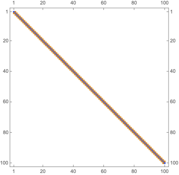
Then we can make the matrix fast:

fdmat[100] // MatrixPlot

Doing the nD extension will take a bit of thought, though.

Partial Solution to Actual Problem

I'm not sure how your actual problem works, but here's a way we can try to build an FD matrix for it using this stuff. The main thing we'll do is break it down into portions with the same dx and dy terms after doing some symbolic pre-simplification. Here's my new setup (same as yours but entirely symbolic):

Clear[r, glass, air, k]
n2 = (Function[{x, y}, #] &@(Simplify`PWToUnitStep@
      PiecewiseExpand@If[x^2 + y^2 <= r^2, glass, air]));
ClearAll[fw, bw, delta]
SetAttributes[#, HoldAll] & /@ {fw, bw};

fw@D[expr_, x_] := 
 With[{\[CapitalDelta] = delta@ToString@x}, 
  Subtract @@ (expr /. {{x -> x + \[CapitalDelta]}, {x -> x}})/\[CapitalDelta]]
bw@D[expr_, x_] := 
 With[{\[CapitalDelta] = delta@ToString@x}, 
  Subtract @@ (expr /. {{x -> x}, {x -> x - \[CapitalDelta]}})/\[CapitalDelta]]

delta[a_ + b_] := delta@a + delta@b
delta[k_. delta[_]] := 0
grad = Function[expr, fw@D[expr, #] & /@ {x, y}];
div = Function[expr, Total@MapThread[bw@D@## &, {expr, {x, y}}]];
elst = e[#][x, y] & /@ Range[2];
baseDiscreteLHS =
  With[{n2 = n2[x, y]}, 
   div@grad@elst + (n2 k^2) elst - grad[div@elst - 1/n2 div[n2 elst]]];

Now I'll prep this stuff so it's in a form my code can use cleanly:

prepped =
  (baseDiscreteLHS[[1]]) //. {
     e[1] -> e1,
     e[2] -> e2,
     delta["y"] -> dy,
     delta["x"] -> dx,
     UnitStep[r^2 - x^2 - y^2] -> usxy,
     UnitStep[r^2 - x^2 - (-dy + y)^2] -> usxdy,
     UnitStep[r^2 - (dx + x)^2 - y^2] -> usdxy,
     UnitStep[r^2 - (dx + x)^2 - (-dy + y)^2] -> usdxdy,
     UnitStep[r^2 - (-dx + x)^2 - y^2] -> usdxmdy
     } // FullSimplify;

Now I'll use this stuff to pull the FD weights just for e1 from the first of the two equations provided:

weightsE1 =
  {
   fdmWeightDataND[prepped[[1]], e1, {x, y}, {dx, dy}],
   fdmWeightDataND[prepped[[2]], e1, {x, y}, {dx, dy}],
   fdmWeightDataND[prepped[[3]], e1, {x, y}, {dx, dy}],
   fdmWeightDataND[prepped[[4]], e1, {x, y}, {dx, dy}],
   fdmWeightDataND[
    Simplify[Collect[prepped[[6]] // Expand, dx][[1]]], 
    e1, 
    {x, y}, 
    {dx, dy}
    ],
   fdmWeightDataND[
    Simplify[Collect[prepped[[8]] // Expand, dx][[1]]], 
    e1,
    {x, y}, 
    {dx, dy}
    ]
   };

Then I'll build all the matrices, add them together, and numericize everything:

mate1 =
 Block[
  {
   r = .8, glass = (1.45)^2, air = 1., k = (2 \[Pi])/1.55,
   sp1, spRules, points = 25,
   dx, dy
   },
  dx = 1./points; dy = 1/points;
  sp1 = FDM2D[#, {dx, dy}, {points, points}] & /@ weightsE1 // Total;
  spRules =
   MapThread[
    # ->
      With[{x = #[[1]]*dx, y = #[[2]]*dy},
       #2 /.
        {
         usxy -> UnitStep[r^2 - x^2 - y^2],
         usxdy -> UnitStep[r^2 - x^2 - (-dy + y)^2],
         usdxy -> UnitStep[r^2 - (dx + x)^2 - y^2],
         usdxdy -> UnitStep[r^2 - (dx + x)^2 - (-dy + y)^2],
         usdxmdy -> UnitStep[r^2 - (-dx + x)^2 - y^2]
         }
       ] &,
    {
     sp1["NonzeroPositions"],
     sp1["NonzeroValues"]
     }
    ];
  SparseArray[spRules, Dimensions[sp1]]
  ]

Finally we can solve this using your same Eigensystem code:

Block[{r = .8, glass = (1.45)^2, air = 1., k = (2 \[Pi])/1.55, points = 25},
  {val, vec} =
   Eigensystem[mate1, -6, Method -> {"Arnoldi", "Shift" -> k^2 glass}
    ];
  mat = ArrayReshape[#, {2, points - 2, points - 2}] & /@ vec;
  MapThread[
   ArrayPlot[#[[1]], PlotLabel -> Sqrt@#2, PlotRange -> All, 
     ColorFunction -> "AvocadoColors"] &,
   {mat, val}
   ]
  ] // AbsoluteTiming

The results are meaningless since I just randomly took part of the problem, but this entire procedure was fast and not memory intensive at all.

Answer 2

To compare code @xzczd and @b3m2a1, I took a simplified version of the 2D operator from the topic here and 300x300 cells. I simplified code @xzczd a little, so it works 3 times faster. Code @b3m2a1, on the contrary, I complicated a little, so that it works 30 times faster. As a result, they now work equally fast and produce the same output.

Code @xzczd

r = .8; glass = (1.45)^2; air = 1.; k = (2 \[Pi])/1.55;
n2[x_, y_] := If[x^2 + y^2 <= r^2, glass, air];
ClearAll[fw, bw, delta]
SetAttributes[#, HoldAll] & /@ {fw, bw};

fw@D[expr_, x_] := 
 With[{\[CapitalDelta] = delta@ToString@x}, 
  Subtract @@ (expr /. {{x -> x + \[CapitalDelta]}, {x -> 
         x}})/\[CapitalDelta]]
bw@D[expr_, x_] := 
 With[{\[CapitalDelta] = delta@ToString@x}, 
  Subtract @@ (expr /. {{x -> x}, {x -> 
         x - \[CapitalDelta]}})/\[CapitalDelta]]

delta[a_ + b_] := delta@a + delta@b
delta[k_. delta[_]] := 0
grad = Function[expr, fw@D[expr, #] & /@ {x, y}];
div = Function[expr, Total@MapThread[bw@D@## &, {expr, {x, y}}]];
elst = e[#][x, y] & /@ Range[1];
discretelhs = 
  With[{n2 = n2[x, y]}, div@grad@elst + (k^2*n2 ) elst] // 
   FullSimplify;
points = 302; L = 2; domain = {-L, L}; grid = 
 Array[# &, points, domain];
del = #[[2 ;; -2]] &;
delta["x"] = delta["y"] = -Subtract @@ domain/(points - 1);
vare = Outer[e[#][#2, #3] &, Range@1, del@grid, del@grid, 1] // 
   Flatten;
discretelhslst = 
   Flatten@Transpose[
     Module[{e}, e[i_][L | -L, _] = e[i_][_, L | -L] = 0.;
      Table[discretelhs, {x, del@grid}, {y, del@grid}]], {2, 3, 
      1}]; // AbsoluteTiming
{barray2, marray2} = 
   CoefficientArrays[discretelhslst, vare]; // AbsoluteTiming
{val, vec} = 
   Eigensystem[marray2, -4, 
    Method -> {"Arnoldi", "Shift" -> k^2 glass}]; // AbsoluteTiming
mat = ArrayReshape[#, {2, points - 2, points - 2}] & /@ vec;
MapThread[
 ArrayPlot[#[[1]], PlotLabel -> Sqrt@#2, PlotRange -> All, 
   ColorFunction -> "AvocadoColors"] &, {mat, val}]

Code @b3m2a1

fdmWeightDataND~SetAttributes~HoldAll;
fdmWeightDataND[a_, dep_Symbol, indeps : {__Symbol}, 
   hs : {__Symbol}] := 
  Block[{dep}, 
   Block[indeps, 
    Block[hs, 
     Module[{weights, order, denomWeight, denom, num, powed, pows, 
       minpow, pts, x}, denom = Denominator[a];
      (*assumes the mesh spacing is in there at different powers*)
      order = Exponent[denom, #] & /@ hs;
      (*pull the power on the mesh spacing*)
      denomWeight = If[order > 0, Coefficient[denom, hs^order], denom];
      num = Numerator[a];
      {powed, pows} = 
       Reap[num /. 
         dep[args___]?(Not@*FreeQ[Alternatives @@ indeps]) :> 
          dep @@ Sow[MapThread[Coefficient[#, #2] &, {{args}, hs}]]];
      minpow = Min[pows];
      weights = 
       AssociationThread[pows[[1]], 
        Map[Coefficient[powed /. (dep @@ #) -> x, x] &, pows[[1]]]];
      <|"Weights" -> weights, "Orders" -> order|>]]]];


FDM2D[weightData_, {hx_, hy_}, {nptsx_, nptsy_}] := 
 Module[{xps, yps, weights = weightData["Weights"], 
   orders = weightData["Orders"]}, 
  xps = Length@DeleteDuplicates@Keys[weights][[All, 1]];
  yps = Length@Sort@DeleteDuplicates@Keys[weights][[All, 2]];
  SparseArray[
    Flatten@KeyValueMap[
      With[{ix = #[[1]], iy = #[[2]], v = #2}, 
        Map[Band[
            If[ix >= 0, {1, 1 + ix}, {1 - ix, 1}] + {#, #} + 
             If[iy >= 0, {0, iy*nptsx}, {-iy*nptsx, 0}], {nptsx*nptsy,
              nptsx*nptsx}, {nptsx, nptsx}] -> v &, 
         Range[nptsx - Abs[ix]] - 1]] &, weights], {nptsx*nptsy, 
     nptsx*nptsx}]/(Times @@ ({hx, hy}^orders))]


ClearAll[fw, bw, delta]
SetAttributes[#, HoldAll] & /@ {fw, bw};

fw@D[expr_, x_] := 
 With[{\[CapitalDelta] = delta@ToString@x}, 
  Subtract @@ (expr /. {{x -> x + \[CapitalDelta]}, {x -> 
         x}})/\[CapitalDelta]]
bw@D[expr_, x_] := 
 With[{\[CapitalDelta] = delta@ToString@x}, 
  Subtract @@ (expr /. {{x -> x}, {x -> 
         x - \[CapitalDelta]}})/\[CapitalDelta]]

delta[a_ + b_] := delta@a + delta@b
delta[k_. delta[_]] := 0
grad = Function[expr, fw@D[expr, #] & /@ {x, y}];
div = Function[expr, Total@MapThread[bw@D@## &, {expr, {x, y}}]];
elst = e[#][x, y] & /@ Range[1];
baseDiscreteLHS = Together[div@grad@elst];
prepped = (baseDiscreteLHS[[1]]) //. {e[1] -> e1, delta["y"] -> dy, 
    delta["x"] -> dx};
weightsE1 = {fdmWeightDataND[prepped, e1, {x, y}, {dx, dy}]};
mate1 = Block[{sp1, spRules, points = 300, dx, dy}, 
    dx = 4./(points + 1); dy = 4./(points + 1);
    sp1 = FDM2D[#, {dx, dy}, {points, points}] & /@ weightsE1 // Total;
    spRules = 
     MapThread[# -> With[{x = #[[1]]*dx, y = #[[2]]*dy}, #2] &, {sp1[
        "NonzeroPositions"], sp1["NonzeroValues"]}];
    SparseArray[spRules, Dimensions[sp1]]]; // AbsoluteTiming
r = .8; glass = (1.45)^2; air = 1.; k = (2 \[Pi])/1.55;
n2[x_, y_] := If[x^2 + y^2 <= r^2, glass, air]; discretelhs = 
 With[{n2 = n2[x, y]}, (k^2*n2) elst];
points1 = 302; L = 2; domain = {-L, L}; grid = 
 Array[# &, points1, domain];
del = #[[2 ;; -2]] &;
delta["x"] = delta["y"] = -Subtract @@ domain/(points1 - 1);
vare = Outer[e[#][#2, #3] &, Range@1, del@grid, del@grid, 1] // 
   Flatten;
discretelhslst = 
  Flatten@Transpose[
    Module[{e}, e[i_][L | -L, _] = e[i_][_, L | -L] = 0.;
     Table[discretelhs, {x, del@grid}, {y, del@grid}]], {2, 3, 1}];
{barray2, marray2} = 
   CoefficientArrays[discretelhslst, vare]; // AbsoluteTiming
points = 300; {val, vec} = 
  Eigensystem[mate1 + marray2, -4, 
   Method -> {"Arnoldi", "Shift" -> k^2*glass}]; // AbsoluteTiming
mat = ArrayReshape[#, {2, points, points}] & /@ vec;
MapThread[
 ArrayPlot[#[[1]], PlotLabel -> Sqrt[#2], PlotRange -> All, 
   ColorFunction -> "AvocadoColors"] &, {mat, val}]

Finally, compare with my method that I suggested for this problem here using FEM:

<< NDSolve`FEM`
r = 0.8; ne = 4;
reg = ImplicitRegion[-2 <= x <= 2 && -2 <= y <= 2, {x, y}];
mesh = ToElementMesh[reg, 
   MeshRefinementFunction -> 
    Function[{vertices, area}, 
     area > 0.0004 (1 + 9 Norm[Mean[vertices]])]];


glass = 1.45; air = 1.; k0 = (2 \[Pi])/1.55; b = I*Sqrt[glass]*k0*1.37;
n[R_] := If[R <= r, glass^2, air^2]*k0^2

helm = -Laplacian[u[x, y], {x, y}] - (b^2 + n[Sqrt[x^2 + y^2]])*
    u[x, y];
boundary = DirichletCondition[u[x, y] == 0, True];

{vals, funs} = 
     NDEigensystem[{helm, boundary}, u[x, y], {x, y} \[Element] mesh, 
    ne]; // AbsoluteTiming
Table[DensityPlot[Im[funs[[i]]], {x, y} \[Element] mesh, 
  PlotRange -> All, 
    PlotLabel -> Im[Sqrt[vals[[i]] + b^2]], Mesh -> None, 
  ColorFunction -> "AvocadoColors", Frame -> True, Axes -> False, 
  FrameTicks -> None], {i, Length[vals]}]

Comparing the data in Figure 1-3, we find that there is an eigenvalue match in methods FDM and FEM. The small difference can be explained by the difference in the number of cells.

Answer 3

I'd like to add my incomplete answer. I call it incomplete because a general-purposed function hasn't been created (yet), but I do find a general strategy for handling the problem.

The idea is simple: generate coefficient array of general difference formula with CoefficientArray first, then generate the complete array using the general coefficients.

I'll solve the 2D problem in the question for illustration. delta, discretelhs etc. are the same as in the question.

sfx = Rescale[#, {x, x + delta@"x"}, {nx, nx + 1}] &;
sfy = Rescale[#, {y, y + delta@"y"}, {ny, ny + 1}] &;
rule = e[i_][x_, y_] :> {i, sfx@x // Simplify, sfy@y // Simplify};
varegeneral = Union@Cases[discretelhs, e[_][__], Infinity];
index = {i, nx, ny, ##} & @@@ (varegeneral /. rule);
coelst = Last@CoefficientArrays[discretelhs, varegeneral];
marrayfast = 
   Flatten[SparseArray[
      Flatten[#, 
          3] &@(Unevaluated@
            Compile[{}, 
             Table[term, {i, 2}, {nx, 2, pts - 1}, {ny, 2, pts - 1}]] /. {term -> index, 
            pts -> points})[] -> (Flatten[#, 
           3] &@(Unevaluated@
             Compile[{}, Table[lst[[i]], {i, 2}, {x, dgrid}, {y, dgrid}]] /. {dgrid -> 
              del@grid, 
             lst -> (Normal@coelst /. {HoldPattern@glass -> glass, 
                 HoldPattern@air -> air})})[]), {2, points, points, 2, points, 
       points}][[All, 2 ;; -2, 2 ;; -2, All, 2 ;; -2, 2 ;; -2]], {{1, 2, 3}, {4, 5, 
      6}}]; // AbsoluteTiming

MaxMemoryUsed[]/1024^2. MB

marrayfast == marray2
(* True *)

{val, vec} = 
   Eigensystem[marrayfast, -6, 
    Method -> {"Arnoldi", "Shift" -> k^2 glass}]; // AbsoluteTiming

MaxMemoryUsed[]/1024^2. MB

mat = ArrayReshape[#, {2, points - 2, points - 2}] & /@ vec;
MapThread[ArrayPlot[#[[1]], PlotLabel -> Sqrt@#2, PlotRange -> All, 
   ColorFunction -> "AvocadoColors"] &, {mat, val}]

When points = 500, it only takes 5.63068 seconds to generate marrayfast, while 53.4027 + 19.1697 to generate marray2.

Memory usage is also reduced, but the real bottleneck seems to be Eigensystem, so perhaps it's not a big deal.