I think I have finally got a method for getting the coefficients of the differential equation. (user21 has been useful as ever).
The starting point is to consider the two equations that are the basis for solving differential equations. From the tutorial: Solving Partial Differential Equations with Finite Elements
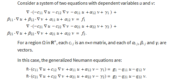
I think there are some typos here . The key point is that in the second set of equations all the terms should be positive while in the system of partial differential equations the corresponding terms should be negative. I also think that the  should be on the right. I am going to call the second equation part1 with coefficients c, α and γ and then the partial differential equation and Neumann equation become

Here part2 are the terms needed to complete the differential equation. The steps I am going to use to derive the equations are as follows. Let me know if there is a simpler method.
- Make a symbolic version of all the needed coefficients.
- Starting from the second equations make a symbolic version of each term .
- Equate these terms to those in the actual equation and make replacement rules for the coefficients. This gives us part1.
- Take the divergence of -part1 and then subtract it from the differential equation to get part2.
- Equate symbolic terms for part2 with the actual terms and thus get replacement rules for these coefficients.
- Generate the coefficients.
- Solve using the coefficients and
InitializePDECoefficients( because I don't know how to make an Inactive version of the differential equation). That can be another question.
Examination of the equations (and some experimentation) shows that we only need c, α, β and a coefficients. The full list of the names of these coefficients are given under InitializePDECoefficients as follows

Here are the equations for the stress and the partial differential equations.
ClearAll[σr,σz,τrz,τzr,σθ]
stress={σr[r,z],τrz[r,z],τzr[r,z],σz[r,z]};
(* ddisp={(u^(1,0))[r,z],(u^(0,1))[r,z],(w^(1,0))[r,z],(w^(0,1))[r,z]}; *)
ddisp = {Derivative[1,0][u][r,z], Derivative[0,1][u][r,z], Derivative[1,0][w][r,z], Derivative[0,1][w][r,z]};
disp={u[r,z],w[r,z]};

(*  stress in terms of strain *)
eqn1={
σr[r,z]==Y/((ν+1) (2 ν-1)) ((ν-1) ϵr-ν (ϵθ+ϵz)),
τrz[r,z]==Y/(2 (1+ν)) γrz,
τzr[r,z]==Y/(2 (1+ν)) γzr,
σz[r,z]==Y/((ν+1) (2 ν-1)) ((ν-1) ϵz-ν (ϵr+ϵθ)),
σθ[r,z]==Y/((ν+1)(2ν-1)) ((ν-1)ϵθ-ν(ϵr+ϵz))
};

(* strain in terms of displacement *)
eqn2={
ϵr-> D[u[r,z],r],
ϵz-> D[w[r,z],z],
ϵθ->u[r,z]/r,
γrz-> D[u[r,z],z]+D[w[r,z],r],
γzr-> D[u[r,z],z]+D[w[r,z],r]
};
(* Get the equations for stress in terms of displacements *)
sol1=First@Solve[eqn1/.eqn2,Join[stress,{σθ[r,z]}]]//Simplify;
(* differential equation to be solved *)
pde={
D[σr[r,z]/.sol1,r]+D[τrz[r,z]/.sol1,z]+(σr[r,z]/r)-σθ[r,z] /r,
D[σz[r,z]/.sol1,z]+D[τzr[r,z]/.sol1,r]+(τzr[r,z]/r)
}/.sol1//Simplify;
Now we have the first step and form the symbolic version of the coefficients and the equations.
n = 2;
space = {r, z};
vars = {u[r, z], w[r, z]};
ccoffs = Array[c, {n, n, n, n}]; (* DiffusionCoefficients *)
αcoffs = Array[α, {n, n, n}];  (* ConservativeConvectionCoefficients *)
βcoffs = Array[β, {n, n, n}];  (* ConvectionCoefficients *)
acoffs = Array[a, {n, n}];   (* ReactionCoefficients *)


cT = Table[Sum[ccoffs[[i, j]].Grad[vars[[j]], space], {j, n}], {i, n}];
αT = Table[Sum[αcoffs[[i, j]] vars[[j]], {j, n}], {i, n}];
βT = Table[Sum[βcoffs[[i, j]].Grad[vars[[j]], space], {j, n}], {i, n}];
aT = Table[Sum[acoffs[[i, j]] vars[[j]], {j, n}], {i, n}];
Next are steps 2 and 3 and a check to see that we have formed part1 correctly
part1 = {{σr[r, z], τrz[r, z]}, {τzr[r,
       z], σz[r, z]}} /. sol1 // Simplify;

{vec1, mat1} = CoefficientArrays[part1, ddisp] // Normal // Simplify;

{vec1S, mat1S} = CoefficientArrays[cT, ddisp] // Normal // Simplify;

sub1 = Thread[Flatten[mat1S] -> Flatten[mat1]];

{vec2, mat2} = CoefficientArrays[part1, disp] // Normal // Simplify;

{vec2S, mat2S} =
  CoefficientArrays[αT, disp] // Normal // Simplify;

sub2 = Thread[Flatten[mat2S] -> Flatten[mat2]];

(* Check we have modeled part1 correctly *)
check1 = cT + αT /. Join[sub1, sub2] // Simplify;

part1 == check1 // Simplify
True
The next step is to find part2. The pde is equal to zero so we can multiply by any value and not change its meaning. Here to fit with the negative value of part1 the pde is multiplied by -1. We get part2 and again match coefficients between symbolic and actual values.
part2 = -pde - Div[-part1, space] // Simplify;

{vec3, mat3} = CoefficientArrays[part2, ddisp] // Normal // Simplify;

{vec3S, mat3S} = CoefficientArrays[βT, ddisp] // Normal // Simplify;

sub3 = Thread[Flatten[mat3S] -> Flatten[mat3]];

{vec4, mat4} = CoefficientArrays[part2, disp] // Normal // Simplify;

{vec4S, mat4S} = CoefficientArrays[aT, disp] // Normal // Simplify;

sub4 = Thread[Flatten[mat4S] -> Flatten[mat4]];

(* Check that part2 is correctly modelled*)
check2 = βT + aT /. Join[sub3, sub4];

part2 == check2 // Simplify
True
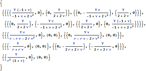
Thus the coefficients are
coffs = {ccoffs, αcoffs, βcoffs, acoffs} /.
  Join[sub1, sub2, sub3, sub4]
Now for an example. First a module to solve the equation.
Needs["NDSolve`FEM`"];
ClearAll[mySolve];
mySolve[{u_, w_}, {r_, z_}, mesh_, ubc_,
  wbc_, {cCoffs_, αCoffs_, βCoffs_, aCoffs_}] := Module[
  {df, ccc, cv, rc, vd, sd, methodData, initCoeffs, initBCs,
   discretePDE, load, stiffness, damping, mass, split, discreteBCs},
  df = "DiffusionCoefficients" -> -cCoffs;
  ccc = "ConservativeConvectionCoefficients" -> -αCoffs;
  cv = "ConvectionCoefficients" -> βCoffs;
  rc = "ReactionCoefficients" -> aCoffs;

  (*variable data*)
  vd = NDSolve`VariableData[{"DependentVariables",
      "Space"} -> {{u, w}, {r, z}}];

  (*Solution data*)
  sd = NDSolve`SolutionData["Space" -> ToNumericalRegion[mesh]];

  (*Initialize the finite element data with the variable and solution \
data.*)
  methodData = InitializePDEMethodData[vd, sd];

  (*Initialize the partial differential equation coefficients.*)
  initCoeffs = InitializePDECoefficients[vd, sd, df, ccc, cv, rc];

  (*Initialize the boundary conditions.*)
  initBCs = InitializeBoundaryConditions[vd, sd, {ubc, wbc}];

  (*Compute the discretized partial differential equation.*)
  discretePDE = DiscretizePDE[initCoeffs, methodData, sd];
  {load, stiffness, damping, mass} = discretePDE["SystemMatrices"];

  (*Compute how the incidents are split between the two dependent \
variables.*)
  {i1, i2, i3} = methodData["IncidentOffsets"];
  split = {i1 + 1 ;; i2, i2 + 1 ;; i3};

  (*Discretize the initialized boundary conditions.*)
  discreteBCs = DiscretizeBoundaryConditions[initBCs, methodData, sd];

  (*Deploy the boundary conditions in place.*)
  DeployBoundaryConditions[{load, stiffness}, discreteBCs];

  {load, stiffness, split}]
Edit
I have changed the answer from here on so that we can have an example which compares a 2D and 3D case. This is at the request of Alex Trounev who would like to make further tests.
The 2D case first
r0 = 1;
r1 = 6;
r2 = 8;
z1 = 5;
z2 = 9;
peram = {Y -> 10^3, ν -> 33/100};
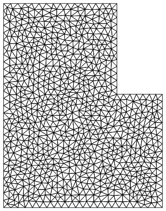
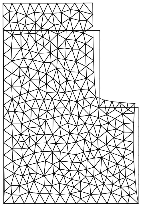
mesh = ToElementMesh[
   RegionUnion[Rectangle[{r0, 0}, {r2, z1}],
    Rectangle[{r0, z1}, {r1, z2}]], MaxCellMeasure -> 0.05];
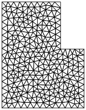
mesh["Wireframe"]
stress = 20;(* stress applied to structure *)

{load, stiffness, split} = mySolve[{u, w}, {r, z}, mesh,
   {DirichletCondition[u[r, z] == 0, z == 0]},
   {DirichletCondition[w[r, z] == 0, z == 0],
    NeumannValue[stress, z == z2]},
   coffs /. peram
   ];
solution = LinearSolve[stiffness, load];
uif = ElementMeshInterpolation[{mesh}, solution[[split[[1]]]]];
wif = ElementMeshInterpolation[{mesh}, solution[[split[[2]]]]];

ClearAll[σz];
σz[r_, z_] := Evaluate[-((Y (ν u[r, z] - r (-1 + ν)
\!\(\*SuperscriptBox[\(w\),
TagBox[
RowBox[{"(",
RowBox[{"0", ",", "1"}], ")"}],
Derivative],
MultilineFunction->None]\)[r, z] + r ν
\!\(\*SuperscriptBox[\(u\),
TagBox[
RowBox[{"(",
RowBox[{"1", ",", "0"}], ")"}],
Derivative],
MultilineFunction->None]\)[r, z]))/(r (1 + ν) (-1 + 2 ν))) /.
    Join[{u -> uif, w -> wif}, peram]];
p11 = Plot[wif[r, z2], {r, r0, r1}, PlotRange -> All,
  PlotStyle -> {Orange}]
p12 = Plot[σz[r, z2], {r, r0, r1},
  PlotRange -> {All, {18, 22}}, PlotRange -> All,
  PlotStyle -> {Orange}]
p13 = Plot[σz[r, z1], {r, r0, r1}, PlotRange -> {All, All},
  PlotRange -> All, PlotStyle -> {Orange}]
p14 = Plot[uif[r2, z], {z, 0, z1}, PlotRange -> All,
  PlotStyle -> {Orange}]
The above will produce plots which we can compare to the 3D case. To make the 3D case we need the mesh as follows
r0 = 1;
r1 = 6;
r2 = 8;
z1 = 5;
z2 = 9;
peram = {Y -> 10^3, ν -> 33/100};
reg1 = BoundaryDiscretizeRegion[Cylinder[{{0, 0, 0}, {0, 0, z1}}, r2]];
reg2 = BoundaryDiscretizeRegion[
   Cylinder[{{0, 0, z1}, {0, 0, z2}}, r1]];
reg3 = RegionUnion[reg2, reg1];
reg4 = BoundaryDiscretizeRegion[Cylinder[{{0, 0, 0}, {0, 0, z2}}, r0]];
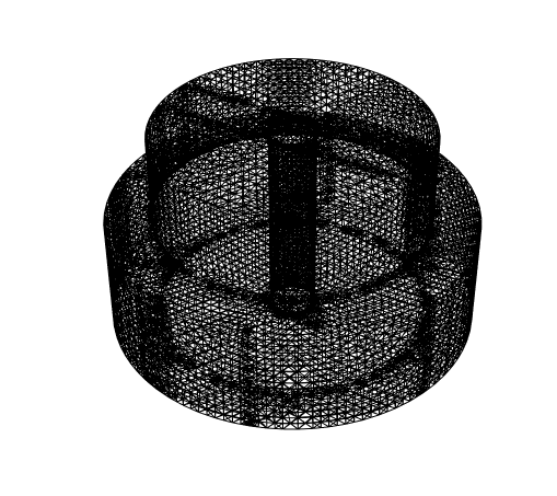
reg = RegionDifference[reg3, reg4]

mesh2 = ToElementMesh[reg, MaxCellMeasure -> 0.1];
mesh2["Wireframe"]
The stress operator is the standard 3D operator
ClearAll[stressOperator];
stressOperator[
  Y_, ν_] := {Inactive[
     Div][{{0, 0, -((Y*ν)/((1 - 2*ν)*(1 + ν)))}, {0, 0,
       0}, {-Y/(2*(1 + ν)), 0, 0}}.Inactive[Grad][
      w[x, y, z], {x, y, z}], {x, y, z}] +
   Inactive[
     Div][{{0, -((Y*ν)/((1 - 2*ν)*(1 + ν))),
       0}, {-Y/(2*(1 + ν)), 0, 0}, {0, 0, 0}}.Inactive[Grad][
      v[x, y, z], {x, y, z}], {x, y, z}] +
   Inactive[
     Div][{{-((Y*(1 - ν))/((1 - 2*ν)*(1 + ν))), 0,
       0}, {0, -Y/(2*(1 + ν)), 0}, {0,
       0, -Y/(2*(1 + ν))}}.Inactive[Grad][
      u[x, y, z], {x, y, z}], {x, y, z}],
  Inactive[Div][{{0, 0, 0}, {0,
       0, -((Y*ν)/((1 -
              2*ν)*(1 + ν)))}, {0, -Y/(2*(1 + ν)),
       0}}.Inactive[Grad][w[x, y, z], {x, y, z}], {x, y, z}] +
   Inactive[
     Div][{{0, -Y/(2*(1 + ν)),
       0}, {-((Y*ν)/((1 - 2*ν)*(1 + ν))), 0, 0}, {0, 0,
       0}}.Inactive[Grad][u[x, y, z], {x, y, z}], {x, y, z}] +
   Inactive[
     Div][{{-Y/(2*(1 + ν)), 0,
       0}, {0, -((Y*(1 - ν))/((1 - 2*ν)*(1 + ν))), 0}, {0,
        0, -Y/(2*(1 + ν))}}.Inactive[Grad][
      v[x, y, z], {x, y, z}], {x, y, z}],
  Inactive[Div][{{0, 0, 0}, {0,
       0, -Y/(2*(1 + ν))}, {0, -((Y*ν)/((1 -
              2*ν)*(1 + ν))), 0}}.Inactive[Grad][
      v[x, y, z], {x, y, z}], {x, y, z}] +
   Inactive[
     Div][{{0, 0, -Y/(2*(1 + ν))}, {0, 0,
       0}, {-((Y*ν)/((1 - 2*ν)*(1 + ν))), 0, 0}}.Inactive[
       Grad][u[x, y, z], {x, y, z}], {x, y, z}] +
   Inactive[
     Div][{{-Y/(2*(1 + ν)), 0, 0}, {0, -Y/(2*(1 + ν)), 0}, {0,
        0, -((Y*(1 - ν))/((1 - 2*ν)*(1 + ν)))}}.Inactive[
       Grad][w[x, y, z], {x, y, z}], {x, y, z}]}

stress = 20;
{uif2, vif2, wif2} = NDSolveValue[{
     stressOperator[Y, ν] == {
       0,
       0,
       NeumannValue[stress , z == z2]},

     DirichletCondition[u[x, y, z] == 0, z == 0],
     DirichletCondition[v[x, y, z] == 0, z == 0],
     DirichletCondition[w[x, y, z] == 0, z == 0]
     } /. peram, {u, v, w}, {x, y, z} ∈ mesh2];

ClearAll[σz1];
σz1[x_,y_,z_]:=Evaluate[(Y ((-1+ν) (w^(0,0,1))[x,y,z]-ν ((u^(1,0,0))[x,y,z]+(v^(0,1,0))[x,y,z])))/((1+ν) (-1+2 ν))/.Join[{u-> uif2,v-> vif2,w-> wif2},peram]];
p21=Plot[Evaluate[Table[wif2[r Cos[θ],r Sin[θ],z2],{θ,0,(19 2π)/20,(2π)/20}]],{r,r0,r1},PlotStyle->{Gray},PlotLegends->LineLegend[{Gray,Orange},{3D,2D}]]
p22=Plot[Evaluate[Table[σz1[r Cos[θ],r Sin[θ],z2],{θ,0,(19 2π)/20,(2π)/20}]],{r,r0,r1},PlotStyle->{Gray},PlotRange->{All,{19.5,20.5}},PlotLegends->LineLegend[{Gray,Orange},{3D,2D}]]
p23=Plot[Evaluate[Table[σz1[r Cos[θ],r Sin[θ],z1],{θ,0,(19 2π)/20,(2π)/20}]],{r,0,r1},PlotStyle->{Gray},PlotRange->All,PlotLegends->LineLegend[{Gray,Orange},{3D,2D}]]
p24=Plot[Evaluate[Table[uif2[r2 Cos[θ],r2 Sin[θ],z]Cos[θ]+vif2[r2 Cos[θ],r2 Sin[θ],z]Sin[θ],{θ,0,(19 2π)/20,(2π)/20}]],{z,0,z2},PlotStyle->{Gray},PlotRange->All,PlotLegends->LineLegend[{Gray,Orange},{3D,2D}]]
Show[p21,p11]
Show[p22,p12]
Show[p23,p13]
Show[p24,p14]
The plots when combined in Show are as follows
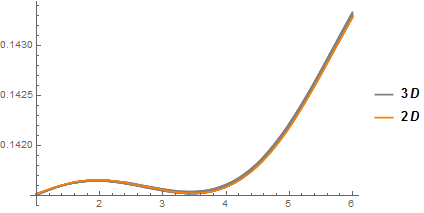
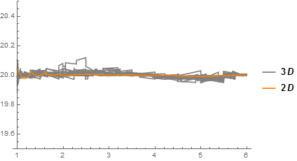
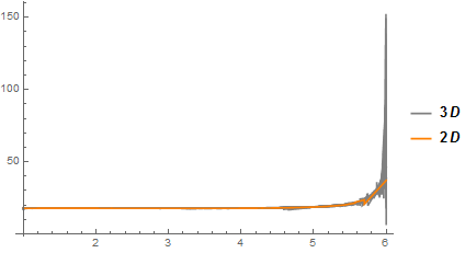
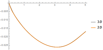
I have plotted the 3D case along a number of lines and all in gray. There is some spread in the 3D values. The 2D plots overlay the 3D ones. The third plots shows some discrepancy at the edge of the region when r = 6. However, this is a stress along a radial line and I don't think it is easy to get the stress directly at the point where the radial line exits the body.
These plots do seem to agree. There is an issue about are the grids compatible for there mesh density? I don't know how do this. Please make comparisons using other code.
The bit I don't know how to do is to put the coefficients into an equation with appropriate Inactivates. Any ideas?
Edit user21:
I deleted my answer; to the best of my knowledge this answer is correct. I am going to show the inactive operator for a top level NDSolveValue call. To do these I usually derive the coefficients, just like you did. The I use 'NDSolve`ProcessEquations' to get the state object and extract the FEM coefficients from that until the inactive form and the coefficients match. I started with
op = {
  Inactive[Div][-coffs[[1, 1, 1]].Inactive[Grad][u[r, z], {r, z}], {r,
     z}],
  Inactive[Div][-coffs[[1, 2, 1]].Inactive[Grad][u[r, z], {r, z}], {r,
     z}]
  }
Evaluated the code below to check that the coefficients match and continued to add terms until I arrived at:
op = {Inactive[
      Div][-coffs[[1, 1, 1]].Inactive[Grad][u[r, z], {r, z}] +
      Inactive[Times][-coffs[[2, 1, 1]], u[r, z]], {r, z}] +
    Inactive[Div][-coffs[[1, 1, 2]].Inactive[Grad][w[r, z], {r, z}] +
      Inactive[Times][-coffs[[2, 1, 2]], w[r, z]], {r, z}] +
    coffs[[3, 1, 1]].Inactive[Grad][u[r, z], {r, z}] +
    coffs[[3, 1, 2]].Inactive[Grad][w[r, z], {r, z}] +
    coffs[[4, 1, 1]]*u[r, z] + coffs[[4, 1, 2]]*w[r, z],
   Inactive[Div][-coffs[[1, 2, 1]].Inactive[Grad][u[r, z], {r, z}] +
      Inactive[Times][-coffs[[2, 2, 1]], u[r, z]], {r, z}] +
    Inactive[Div][-coffs[[1, 2, 2]].Inactive[Grad][w[r, z], {r, z}] +
      Inactive[Times][-coffs[[2, 2, 2]], w[r, z]], {r, z}] +
    coffs[[3, 2, 1]].Inactive[Grad][u[r, z], {r, z}] +
    coffs[[3, 2, 2]].Inactive[Grad][w[r, z], {r, z}] +
    coffs[[4, 2, 1]]*u[r, z] + coffs[[4, 2, 2]]*w[r, z]
   };
This is the proposed inactive form of the operator and I check that it matches the input coefficients by extracting them from the state object.
{state} =
  NDSolve`ProcessEquations[{op == {0,
       NeumannValue[stress, z == z2]} /. peram,
    DirichletCondition[{u[r, z] == 0, w[r, z] == 0}, z == 0]}, {u,
    w}, {r, z} \[Element] mesh];
pdecd = state["FiniteElementData"]["PDECoefficientData"];
Setup:
numCoff = coffs /. peram;
Check:
numCoff[[1]] // MatrixForm
pdecd["DiffusionCoefficients"] // MatrixForm

numCoff[[2]] // MatrixForm
pdecd["ConservativeConvectionCoefficients"] // MatrixForm

numCoff[[3]] // MatrixForm
pdecd["ConvectionCoefficients"] // MatrixForm

numCoff[[4]] // MatrixForm
pdecd["ReactionCoefficients"] // MatrixForm
The sign differece in the first two is OK, since that is added when given to InitializePDECoefficients. The structural difference in the third coefficient is also nothing to worry about. It's just the internal representation that differs from the input form.
We can then use:
{uifND, wifND} =
  NDSolveValue[{op == {0, NeumannValue[stress, z == z2]} /. peram,
    DirichletCondition[{u[r, z] == 0, w[r, z] == 0}, z == 0]}, {u,
    w}, {r, z} \[Element] mesh];
And get:
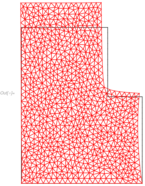
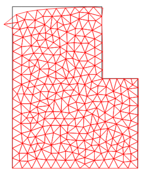
Show[{mesh["Wireframe"["MeshElement" -> "BoundaryElements"]],
  ElementMeshDeformation[mesh, {uifND, wifND}, "ScalingFactor" -> 10][
   "Wireframe"[
    "ElementMeshDirective" -> Directive[EdgeForm[Red], FaceForm[]]]]}]
This is the same result one gets when using the low level FEM functions as above. A final note, the operator op above has terms resulting in zero when looked at closely, but I wanted to show how such an inactive version of the operator would look in a more general scenario.


 should be on the right. I am going to call the second equation part1 with coefficients c, α and γ and then the partial differential equation and Neumann equation become


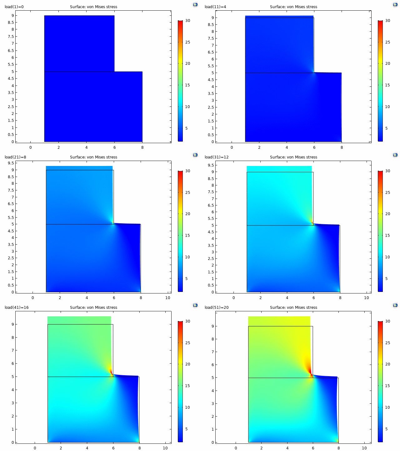

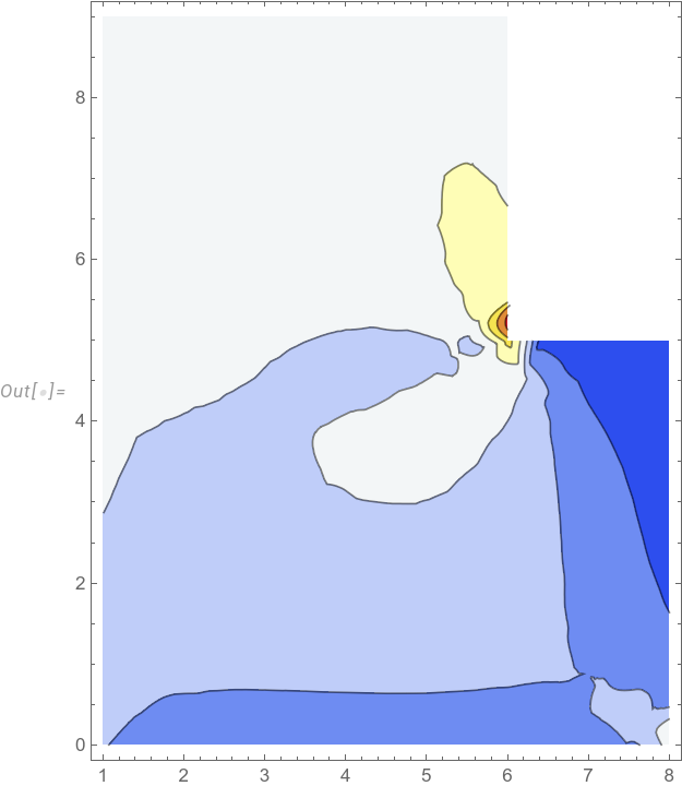
factor * {{-1 + nu, -nu, -nu, 0}, {-nu, -1 + nu, -nu, 0}, {-nu, -nu, -1 + nu, 0}, {0, 0, 0, (-1 + 2*nu)/2}}with factor beingY/((1 + nu)*(-1 + 2*nu)). I am familiar with{{-1 + nu, nu, nu, 0}, {nu, -1 + nu, nu, 0}, {nu, nu, \[Nu]1, 0}, {0, 0, 0, (1 - 2*nu)/2}}with factorY/((1 - 2*nu)*(1 + nu)). Do you recall where you go your form from? $\endgroup$