The data given here
data = Table[Clip[Sin[x], {0, 1}], {x, 0, 2 \[Pi], 0.1}]
generates the following curve
ListPlot[data]
I want to know, how to compute the integral of this curve using only the data given above.
The data given here
data = Table[Clip[Sin[x], {0, 1}], {x, 0, 2 \[Pi], 0.1}]
generates the following curve
ListPlot[data]
I want to know, how to compute the integral of this curve using only the data given above.
Assuming the stepsize is 0.1 as suggested by the construction of the Table, you can calculate:
0.1*Total[data]
to get the numerical integral. To visualize the integral and plot it you can ListPlot:
0.1*Accumulate[data]
Hence:
data = Table[Clip[Sin[x], {0, 1}], {x, 0, 2 \[Pi], 0.1}];
ListPlot[{data, 0.1*Accumulate[data]}]
Using Tai's method:
ω = ConstantArray[0.1, Length[data]];
ω[[1]] *= 0.5;
ω[[-1]] *= 0.5;
ω.data
Alternatively
a = Table[{x, Clip[Sin[x], {0., 1.}]}, {x, 0, 2 π, 0.1}];
Integrate[Interpolation[a][x], {x, a[[1, 1]], a[[-1, 1]]}]
2.00038
Interpolation you can also play with the InterpolationOrder option to increase the accuracy (sometimes). In this case it doesn't do much though.
$\endgroup$
It seems that Simpson's rule has not been mentioned yet, which is the result from a 2nd-order interpolation and will have a smaller error than that from a 1st-order one. So according to the formula, the inputs are the List of samples of the function data and the step size h:
simpsoncoefficients[n_] := SparseArray[{1 -> 1, -1 -> 1, i_?EvenQ -> 4}, n, 2]
integral[data_, h_] := (h/3) simpsoncoefficients[Length[#]].# &[data]
Then integral[data, 0.1] gives 2.00024.
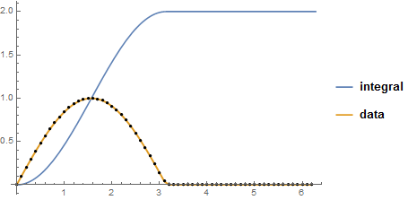
You mention that you want the integral as a plot in a comment; I wonder if the following is what you had in mind. Here I am using your definition of data, and assuming a $0.1$ step size, as hinted at by your Table expression.
tuples = Transpose@{Range[0, 2 Pi, 0.1], data};

Show[
  Plot[
    NIntegrate[Interpolation[tuples][x], {x, 0, xmax}, Method -> "Trapezoidal"],
    {xmax, 0, 2 Pi}, PlotLegends -> {"integral"}
  ],
  ListPlot[
    Style[tuples, Thick, ColorData[97][2]],
    Mesh -> All, MeshStyle -> Directive[Black, PointSize[0.01]],
    PlotLegends -> {"data"}, Joined -> True
  ]
]
