When manipulating B-splines in this manner, it is often convenient to fall back on the definitions. Luckily, since Mathematica supplies the function BSplineBasis[], using the definitions are easy:
pts = {{0, 0}, {1, 1}, {2, -1}, {3, 0}, {4, -2}, {5, 1}};

n = 3; (* B-spline degree *)
m = Length[pts];
(* clamped uniform knots for B-spline *)
knots = {ConstantArray[0, n + 1], Range[m - n - 1]/(m - n), ConstantArray[1, n + 1]}
        // Flatten;

{xu, yu} = Transpose[pts];
bs = BSplineFunction[pts, SplineDegree -> n];

(* B-spline component functions *)
f[t_] = xu.Table[BSplineBasis[{n, knots}, i - 1, t], {i, Length[pts]}];
g[t_] = yu.Table[BSplineBasis[{n, knots}, i - 1, t], {i, Length[pts]}];
Compare:
{ParametricPlot[bs[t], {t, 0, 1}, Axes -> None, Frame -> True,
                Epilog -> {Directive[AbsolutePointSize[5], Red], Point[pts]}],
 ParametricPlot[{f[t], g[t]}, {t, 0, 1}, Axes -> None, Frame -> True,
                Epilog -> {Directive[AbsolutePointSize[5], Red], Point[pts]}]}

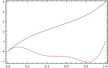
One can now plot the component functions as needed:
Plot[{f[t], g[t]}, {t, 0, 1}, Axes -> None, Frame -> True]

or use derivatives:
With[{t = 1/3}, g''[t]/Sqrt[f'[t]^2 + g'[t]^2]]
   48/Sqrt[41]


