24
$\begingroup$
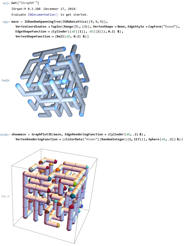
Get["IGraphM`"]
maze = IGRandomSpanningTree[IGMakeLattice[{5, 5, 5}], 
  VertexCoordinates -> Tuples[Range[5], {3}], VertexShape -> None, 
  EdgeStyle -> CapForm["Round"], 
  EdgeShapeFunction -> (Cylinder[{#1[[1]], #1[[2]]}, 0.2] &), 
  VertexShapeFunction -> (Ball[#1, 0.2] &)]
showmaze = 
 GraphPlot3D[maze, EdgeRenderingFunction -> (Cylinder[#1, .2] &), 
  VertexRenderingFunction -> ({ColorData["Atoms"][
       RandomInteger[{1, 117}]], Sphere[#1, .2]} &)]

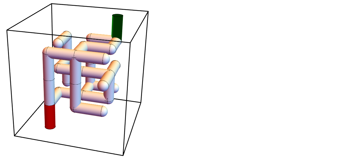
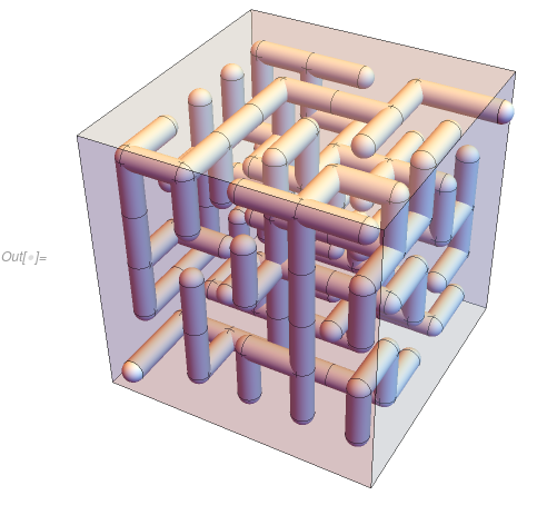
enter image description here

I've generated the bone of a maze here, but I want to make it carved out in a cube, so it's really a maze.

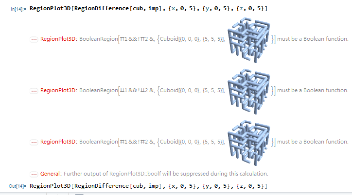
I've tried (1) Exporting showmaze to stl, re-importing to get a MeshRegion(which I don't know how to display), and apply RegionDifference enter image description here

but it fails. enter image description here

(2) Try to make a hole from the showmaze, but I cannot find any reference on how to do this.

$\endgroup$
1
  • 3
    $\begingroup$ If you want people to run your code post it as text, not images; the latter are too difficult to cut and paste into a notebook. $\endgroup$ Commented Feb 7, 2019 at 8:59

4 Answers 4

25
+50
$\begingroup$

Here's an approach that unions the primitives as rasters, meshes, and smooths.

Data from OP:

showmaze = Uncompress[FromCharacterCode @@ ImageData[Import["https://i.sstatic.net/XVJcP.png"], "Byte"]];

Primitives with an extended inlet and outlet:

prims = CapsuleShape @@@ Cases[showmaze, _Cylinder, ∞];
prims = prims /. {{5., 5., 5.} -> {5.5, 5., 5.}, {1., 1., 1.} -> {1., 0.5, 1.}};

Now let's rasterize the model. To ensure a quality rasterization, I'll rasterize each capsule separately and join them together:

ims = RegionImage[#, {{0.3`, 5.7`}, {0.3`, 5.7`}, {0.3`, 5.7`}}, RasterSize -> 100] & /@ prims;
im = ImageApply[Max, ims]
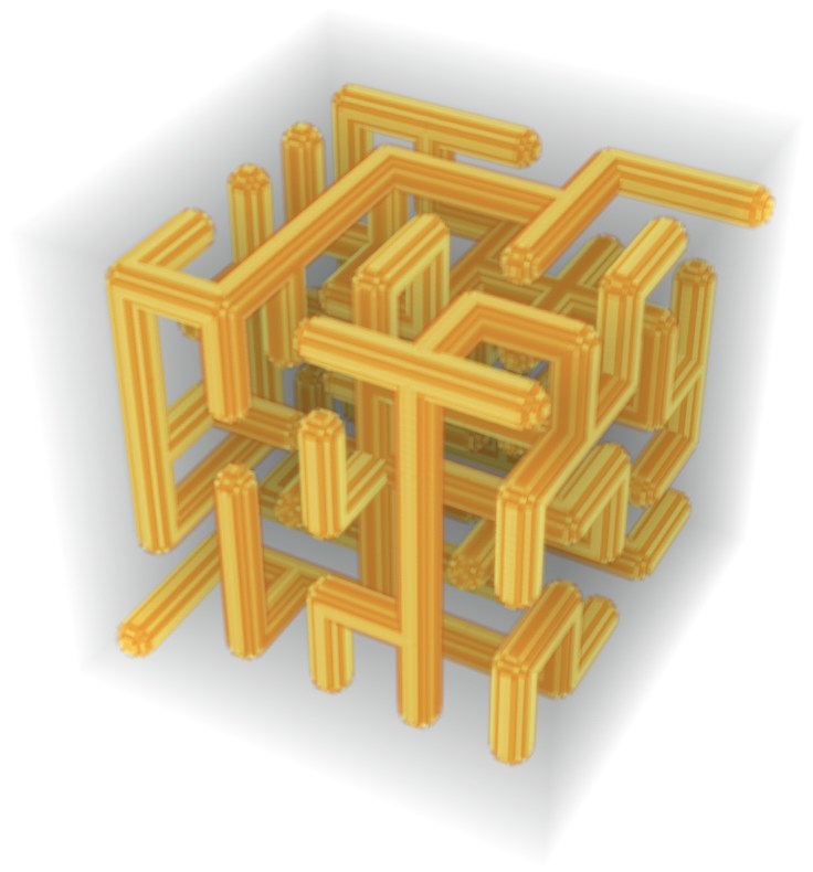
We'd like the complement of this image:

im = ImageTake[ColorNegate[im], {5, -5}, {5, -5}, {5, -5}]
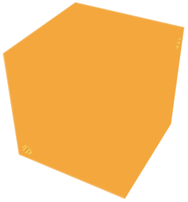
Now mesh the data. Here I've clipped to show inside:

Show[bmr = ImageMesh[im, Method -> "DualMarchingCubes"], PlotRange -> {{0, 91}, {1, 92}, {0, 91}}]
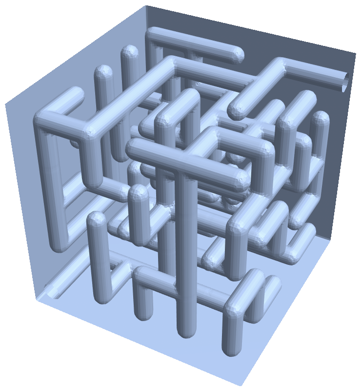
This looks pretty good, and for applications like 3D printing it’s very much sufficient, but there are some artifacts we could smooth. One approach is to use GraphDiffusionFlow defined here, but I was unable to find parameters that smoothed out the caps nicely.

Instead I've gone ahead and implemented a version of the approach outlined here. The code for this is at the bottom of the post.

cube = smoothMeshRegion[bmr];

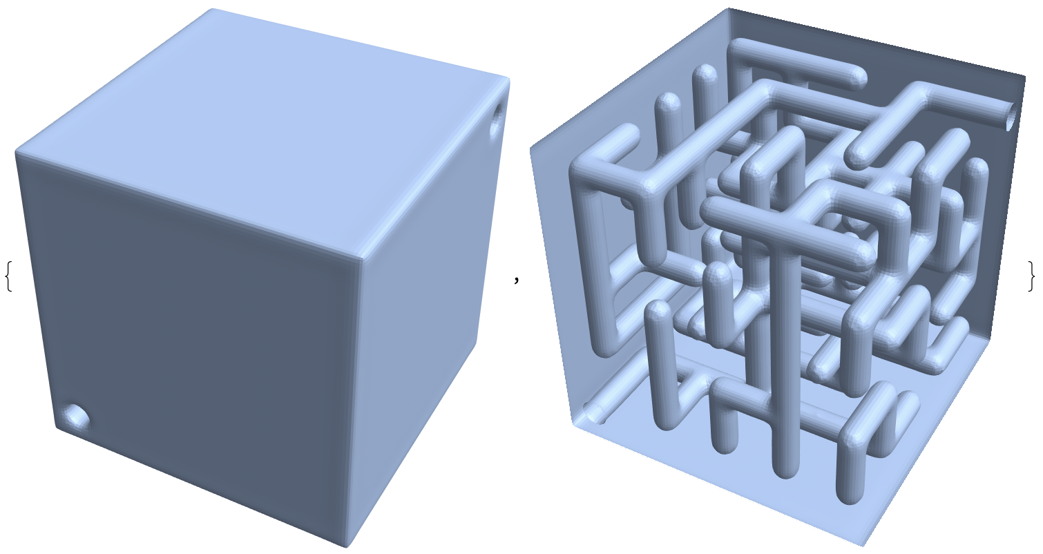
This looks a bit better, however the outer part of the cube has very soft edges:

{cube, Show[cube, PlotRange -> {{-1, 91}, {1, 93}, {-1, 91}}]}
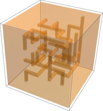
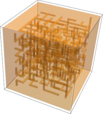
enter image description here

We can fix this by clipping:

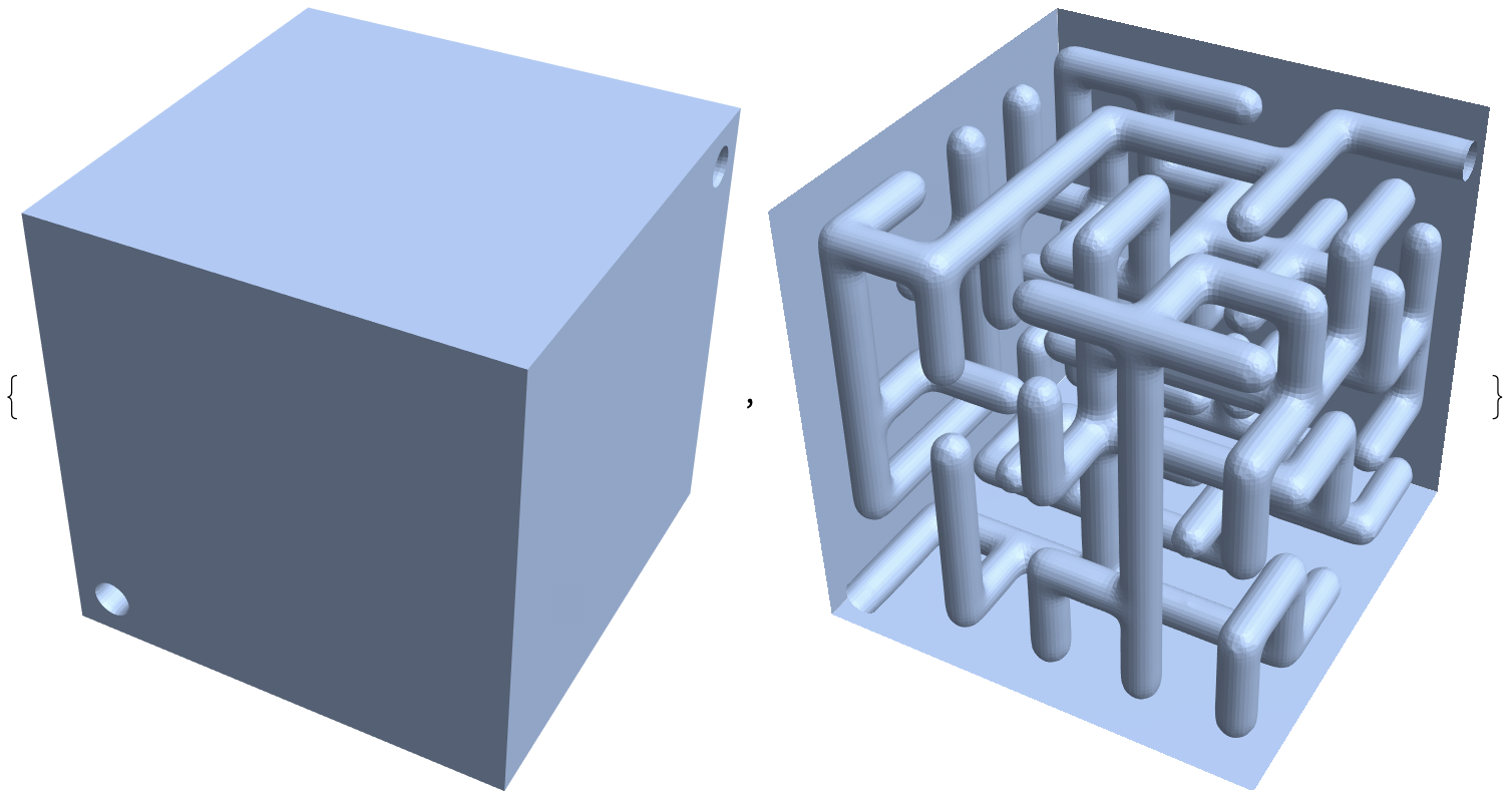
cube = BoundaryDiscretizeRegion[smoothed, {{1, 91}, {1, 91}, {1, 91}}];

{cube, Show[cube, PlotRange -> {{1, 90}, {2, 91}, {1, 90}}]}
enter image description here

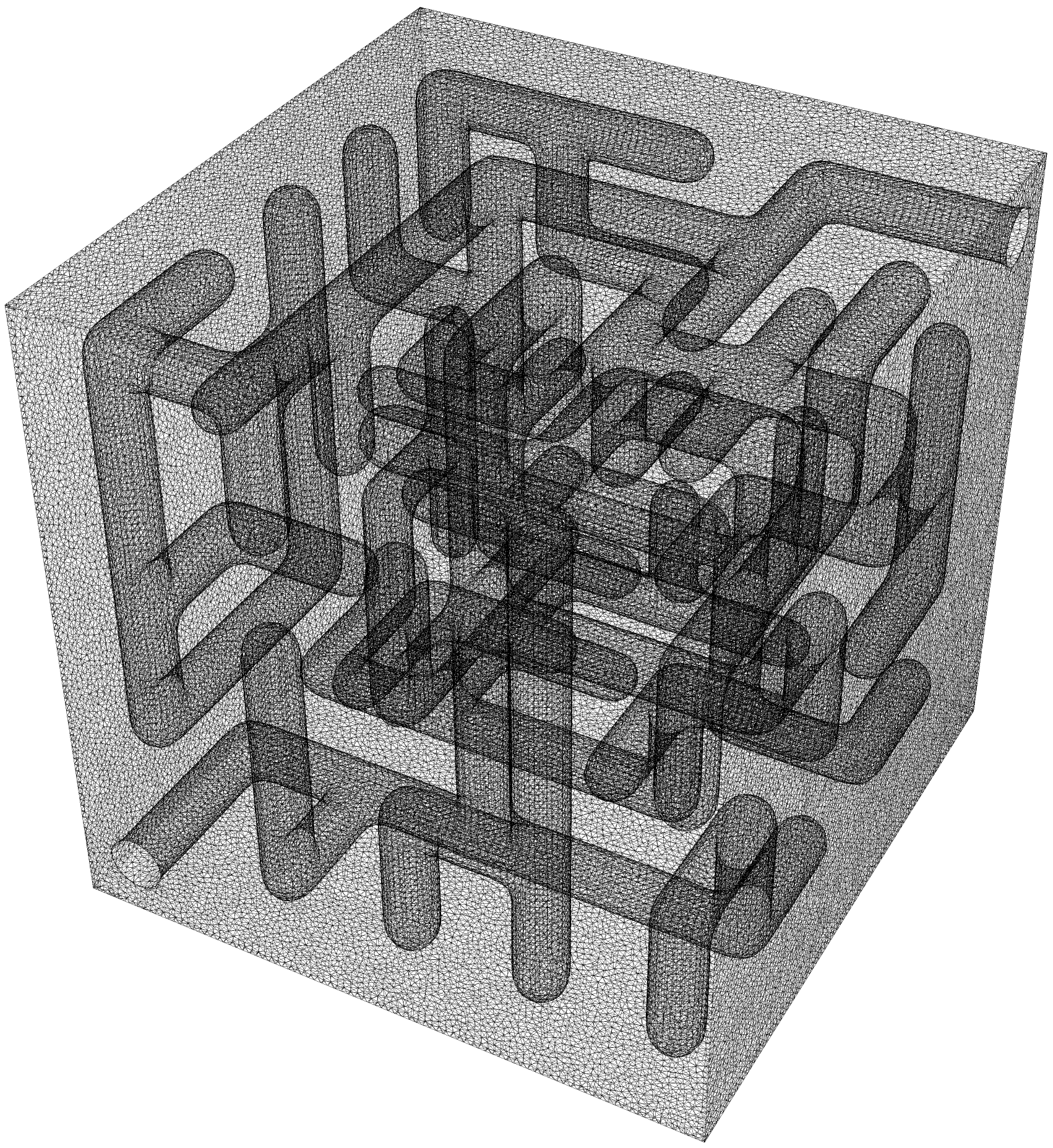
Finally a wireframe view:

BoundaryMeshRegion[cube, MeshCellStyle -> {1 -> {Thin, Black}}, PlotTheme -> "Lines"]

Edit

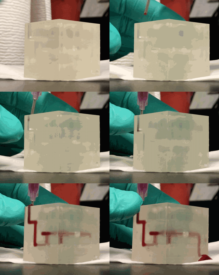
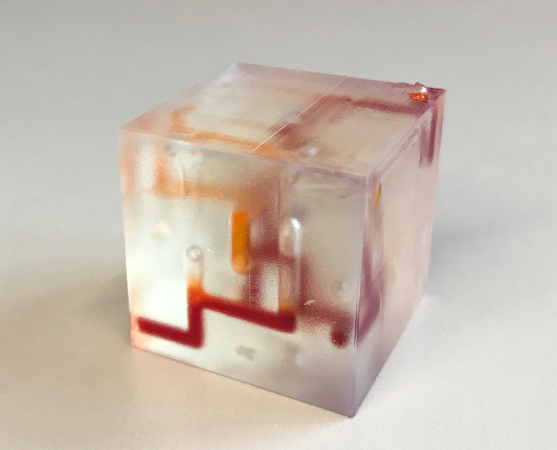
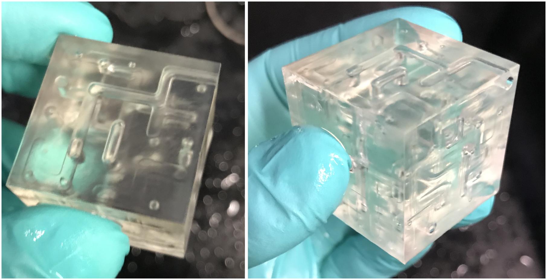
I couldn't resist printing this maze
enter image description here

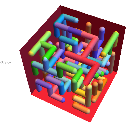
and solving it with food coloring.

enter image description here

enter image description here


Code Dump

(* https://pdfs.semanticscholar.org/c04a/52ad1287385b18464b61f190d1888bf95efd.pdf
   Note: the paper suggests to work with the face centroids. I saw no discernible difference between using them or just the face vertices, so for speed and ease of implementation I'm going with the former.  *)

Options[smoothMeshRegion] = {"FeatureVertices" -> Automatic, "LaplacianMatrixMethod" -> Automatic, "VertexPenalty" -> Automatic};

smoothMeshRegion[mr:(_MeshRegion|_BoundaryMeshRegion), OptionsPattern[]] :=
    Block[{coords, cells, n, L, findices, Fdiag, μ, F, m, A, b, At, ncoords},

        (* ------------ mesh data ------------ *)

        coords = MeshCoordinates[mr];
        cells = MeshCells[mr, 2, "Multicells" -> True];
        n = Length[coords];

        (* ------------ Laplacian matrix ------------ *)

        Switch[OptionValue["LaplacianMatrixMethod"],
            "UniformWeight", L = UniformWeightLaplacianMatrix[mr],
            Automatic|"Contangent"|_, L = CotangentLaplacianMatrix[mr]
        ];

        (* ------------ vertex penalty matrix ------------ *)

        {findices, μ} = featureVertices[mr, OptionValue["FeatureVertices"]];

        Fdiag = vertexPenalty[coords, OptionValue["VertexPenalty"]];
        Fdiag = ReplacePart[Fdiag, Thread[findices -> μ]];

        F = DiagonalMatrix[SparseArray[Fdiag]];
        m = Length[F];

        (* ------------ global matrix ------------ *)

        A = Join[L, F];

        (* ------------ right hand side ------------ *)

        b = ConstantArray[0., {Length[A], 3}];
        b[[n + 1 ;; n + m]] = Fdiag * coords;

        (* ------------ solve the system ------------ *)

        At = Transpose[A]; 
        ncoords = Quiet[LinearSolve[At.A, At.b, Method -> "Pardiso"]];

        (* for large enough μ, ensure the feature vertices are truly fixed *)
        If[TrueQ[μ >= $μ],
            ncoords[[findices]] = coords[[findices]]
        ];

        (* ------------ construct mesh ------------ *)

        Head[mr][ncoords, cells]
    ]

CotangentLaplacianMatrix[mr_] :=
    Block[{n, cells, prims, p1, p2, cos, cots, inds, spopt, L},
        n = MeshCellCount[mr, 0];
        cells = MeshCells[mr, 2, "Multicells" -> True][[1, 1]];
        prims = MeshPrimitives[mr, 2, "Multicells" -> True][[1, 1]];

        p1 = prims - RotateRight[prims, {0, 1}];
        p2 = -RotateRight[p1, {0, 1}];
        cos = Total[p1 p2, {3}] Power[Total[p1^2, {3}]*Total[p2^2, {3}], -0.5];
        cots = .5Flatten[cos*Power[1 - cos^2, -.5]];

        inds = Transpose[{Flatten[cells], Flatten[RotateLeft[cells, {0, 1}]]}];

        Internal`WithLocalSettings[
            spopt = SystemOptions["SparseArrayOptions"];
            SetSystemOptions["SparseArrayOptions" -> {"TreatRepeatedEntries" -> Total}],
            L = SparseArray[inds -> cots, {n, n}],
            SetSystemOptions[spopt]
        ];

        L = L + Transpose[L];
        L = L - SparseArray[{Band[{1, 1}] -> Total[L, {2}]}];

        L
    ]

UniformWeightLaplacianMatrix[mr_] :=
    Block[{C00, W, II},
        C00 = Unitize[#.Transpose[#]]&[mr["ConnectivityMatrix"[0, 2]]];
        W = SparseArray[-Power[Map[Length, C00["MatrixColumns"]] - 1, -1.0]];
        II = IdentityMatrix[Length[C00], SparseArray];

        SparseArray[(C00 - II)W + II]
    ]

$μ = 5.0;
$λ = 0.5;

featureVertices[mr_, fv:Except[{_, _?Positive}]] := featureVertices[mr, {fv, $μ}];
featureVertices[_, {None, μ_}] := {{}, μ};
featureVertices[mr_, {Automatic, μ_}] := {Union @@ Region`InternalBoundaryEdges[mr][[All, 1]], μ}
featureVertices[_, {vinds_, μ_}] /; VectorQ[vinds, IntegerQ] && Min[vinds] <= 1 := {vinds, μ}
featureVertices[_, {_, μ_}] := {{}, μ};

vertexPenalty[coords_, λ:(Automatic|_?NumericQ)] := ConstantArray[If[TrueQ[NonNegative[λ]], λ, $λ], Length[coords]]
vertexPenalty[coords_, vpfunc_] := vpfunc[coords]
$\endgroup$
7
  • $\begingroup$ @Hurst: I produced all of the above output, except the last line (BoundaryMeshRegion[cube, ...]) produced a black square brick. Do you have any idea what could be wrong? $\endgroup$
    – CElliott
    Commented Feb 13, 2019 at 21:23
  • $\begingroup$ It's a slightly large mesh and so the line thicknesses might be blending together on your screen. Try adding in ImageSize -> 1024 or some similar large value. $\endgroup$
    – Greg Hurst
    Commented Feb 13, 2019 at 21:25
  • 1
    $\begingroup$ That was the answer, only the image is still fairly dark. I used ImageSize -> (1024+512) and it looks more nearly like yours only much bigger. Thanks. $\endgroup$
    – CElliott
    Commented Feb 13, 2019 at 21:48
  • $\begingroup$ @ChipHurst A+ GIF (and of course A+ answer) $\endgroup$
    – b3m2a1
    Commented Feb 14, 2019 at 4:42
  • 1
    $\begingroup$ Thanks. It was on an SLA printer. $\endgroup$
    – Greg Hurst
    Commented Feb 14, 2019 at 15:57
25
+200
$\begingroup$

Lets start by making a symbolic representation of maze, with BooleanRegion using graphic primitives. That will be our basis for discretization by any method. Number of vertices of graph should be small to make experimentation easier.

(* "IGraphM" package downloaded from https://github.com/szhorvat/IGraphM *)
Get["IGraphM`"]

n = 3; (* Number of vertices per dimension. *)

IGSeedRandom[42]; (* Set random seed for repeatability. *)
mazeGraph = IGRandomSpanningTree[
  IGMakeLattice[{n, n, n}],
  VertexCoordinates -> Tuples[Range[n], {3}]
]

maze = GraphPlot3D[
  (* Convert it to directed graph, to avoid double rendering of edges. *)
  DirectedGraph[mazeGraph, "Acyclic"],
  EdgeRenderingFunction -> (Cylinder[#1, .2] &),
  VertexRenderingFunction -> (Ball[#1, .2] &),
  Axes -> True
]

Add definition for outer box, entry point and exit point. Then show them together with maze graphics.

cuboid = Cuboid[{0., 0., 0.}, (n + 1) {1., 1., 1.}];
entry = Cylinder[{{1., 1., 0.}, {1., 1., 1.}}, 0.2];
exit = Cylinder[{{n, n, n}, {n, n, n + 1}}, 0.2];

Show[
 Graphics3D[{FaceForm[Red], entry, FaceForm[Green], exit}],
 Graphics3D[{EdgeForm[Directive[Thick, Black]], FaceForm[], cuboid}],
 maze,
 Boxed -> False
]

MazeGraphics

Extract a list of graphic primitives Cylinder and Ball.

primitives = Join[
  Cases[maze, _Cylinder | _Ball, Infinity],
  {entry, exit}
];

Create symbolic BooleanRegion where each primitive is subtracted from outer box.

reg = Fold[
   RegionDifference,
   cuboid,
   primitives
]

Here I have tried to use functions BoundaryDiscretizeRegion and DiscretizeRegion on reg with different option values for Method and AccuracyGoal but nothing worked. It seems to me that currently Mathematica (v11.3) can't handle discretization of such (complex) 3D regions.


I can offer alternative solution which uses Gmsh software for discretization our BooleanRegion. I have created package GmshLink with very basic functionality, but just enough to solve our problem.

(* Load the package and then set path to Gmsh executable. *)
Get["GmshLink`"]
$GmshDirectory = "local/path/to/directory/with/gmsh.exe";

Then use ToElementMesh function with custom mesh generating function GmshGenerator.

mesh = ToElementMesh[
  reg,
  RegionBounds[cuboid],
  "BoundaryMeshGenerator" -> None,
  "ElementMeshGenerator" -> {GmshGenerator, "OptimizeQuality" -> False},
  MaxCellMeasure -> 0.2
]

It produces tetrahedral mesh of decent quality (for FEM purposes). "OptimizeQuality" can be set to True to get mesh with better quality, but this takes more time.

Through[{Min, Mean}@Flatten[mesh["Quality"]]]
(* {0.165972, 0.724565} *)

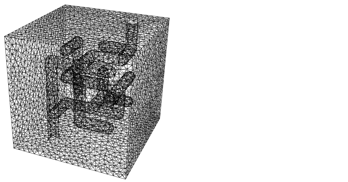
mesh["Wireframe"]

MazeMesh1

Discretization via Gmsh is not too slow and I think it would be possible to create maze for n=5, just go easy on MaxCellMeasure. Resulting ElementMesh can be converted to to MeshRegion if neccesary.

mr = MeshRegion[mesh]

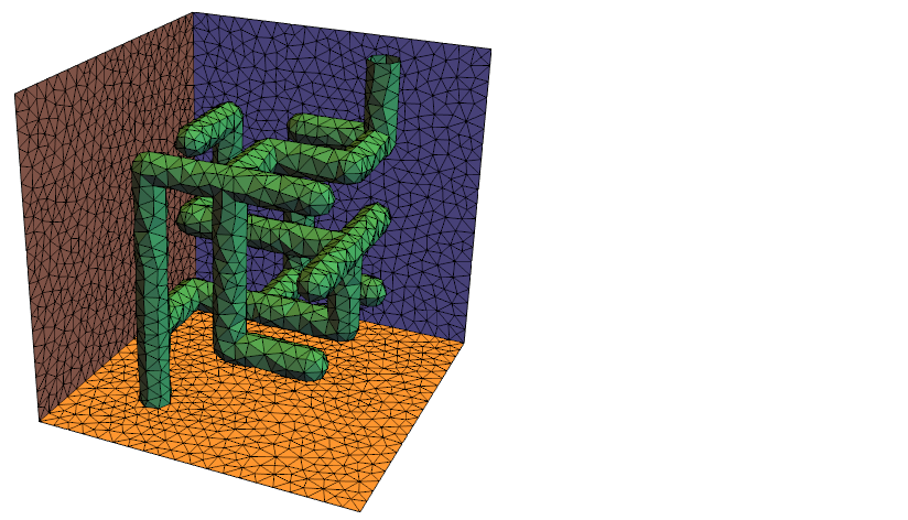
We can group "BoundaryElements" according to their normals, assign markers to them and use this for nice visualization.

applyBoundaryMarkers[mesh_ElementMesh,tolerance_?NumberQ]:=Module[
    {grouping,bElms,markers},

    grouping=GroupBoundariesByNormals[mesh,Clip[tolerance,{0,1}]];
    bElms=First[mesh["BoundaryElements"]];
    markers=ReplaceAll[
        Range@First[grouping],
        Dispatch@(Join@@MapIndexed[
            Thread[#1->First[#2]]&,
            Last[grouping]
        ])
    ];

    ToElementMesh[
        "Coordinates"->mesh["Coordinates"],
        "MeshElements"->mesh["MeshElements"],
        "BoundaryElements"->{Head[bElms][ElementIncidents@bElms,markers]},
        "PointElements"->mesh["PointElements"]
    ]
]

Use the above defined function on tetrahedral mesh. Grouping tolerance is adjusted manually.

meshWithMarkers = applyBoundaryMarkers[mesh, 0.5];
meshWithMarkers["BoundaryElementMarkerUnion"]
(* {1, 2, 3, 4, 5, 6, 7} *)

meshWithMarkers["Wireframe"[
  Or @@ Thread[ElementMarker == {1, 4, 5, 7}],
  "MeshElement" -> "BoundaryElements",
  "MeshElementStyle" -> FaceForm@*Lighter /@ ColorData[112, "ColorList"]
]]

MazeMesh2

$\endgroup$
8
  • 2
    $\begingroup$ This is great! Note that you need to condition your code on $OperatingSystem in a few places. On MacOS, the executable is simply gmsh, not gmsh.exe. Also the function quotes is not needed for Unix based operating systems, so If[$OperatingSystem === "Windows", quotes[str_String]:="\""<>str<>"\""; quotes[other_]:=other, quotes = Identity]; $\endgroup$
    – Greg Hurst
    Commented Feb 8, 2019 at 1:22
  • $\begingroup$ Awesome! Keep up the good work! $\endgroup$
    – user21
    Commented Feb 8, 2019 at 6:20
  • 2
    $\begingroup$ @ChipHurst pointed out that you can shave off some time by setting "BoundaryMeshGenerator"->None if you do not make use of the "BoundaryMesh" in the numerical region in the interface. $\endgroup$
    – user21
    Commented Feb 8, 2019 at 10:19
  • $\begingroup$ This answer is more than what I was expecting, but when I tried to add an entrance and exit, it stopped working, halting at the evaluation. The mesh generation is for FEM, and probably overkill/too complicated for general processing, and I'm hoping that there is still a better method. $\endgroup$
    – seilgu
    Commented Feb 9, 2019 at 18:31
  • 1
    $\begingroup$ "BoundaryMeshGenerator" -> None, "ElementMeshGenerator" -> {GmshGenerator, "OptimizeQuality" -> False}, These are new? Now it's a lot faster. Thanks! $\endgroup$
    – seilgu
    Commented Feb 11, 2019 at 9:21
10
$\begingroup$

OK, I just learned a bunch from the question and @Pinti's answer, thanks!

As an experiment, this generates a maze with rectangular passageways. The good news is you can stay in Mathematica to the finish line. Start same as @Pinti, but just generate the maze, not worrying about cylinders.

n = 4;
maze = IGRandomSpanningTree[IGMakeLattice[{n, n, n}], VertexCoordinates -> Tuples[Range[n], {3}]];

Grab the adjacency list and the positions of the vertices, and get a list of undirected edges. I am sure I am kludging this. Also set the "radius" for the passageways.

al = AdjacencyList[maze];
vs = (AbsoluteOptions[maze, VertexCoordinates] // Values // First);
undir = Union@(Sort /@ Flatten[MapIndexed[Outer[List, ##] &, al], 2]);
radius = .1

Get the cuboids that follow the edges. They currently overlap each other.

cubmazeInner = Map[
              Cuboid[vs[[First@#]] - radius {1, 1, 1}, vs[[Last@#]] + radius {1, 1, 1}] &, 
              undir, 1];

Define the entry, exit, and enveloping cuboid as per @Pinti, and add the entry and exit to the list of Cuboids that make the maze.

entry = Cuboid[{1., 1., 0.} - radius {1, 1, 1}, {1., 1., 1.} + radius {1, 1, 1}];
exit = Cuboid[{n, n, n} - radius {1, 1, 1}, {n, n, n + 1} + radius {1, 1, 1}];
cuboid = Cuboid[{0, 0, 0}, (n + 1) {1, 1, 1}];

cubmaze = Join[cubmazeInner, {entry, exit}];

Take a look. Reminds me of where people pour molten metal into ant colonies.

res = BooleanRegion[Or, cubmaze];
Show[
    Graphics3D[res],
    Graphics3D[{EdgeForm[Directive[Thick, Black]], FaceForm[], cuboid}],
    Boxed -> False]

enter image description here

Probably because of the cuboidal nature of the geometry, Mathematica can get us all the way to the finish line at this point. Using @Pinti's method, which did not work for the cylindrical passageways...

reg = Fold[RegionDifference, cuboid, cubmaze];

RegionPlot3D[reg, PlotStyle -> Opacity[0.3]]

enter image description here

You can spin it around and see inside it. Very cool. Exported it to STL and imported it to CAD, and it looks fine. Tempted to try to print one.

Note that this did not work...

internals = RegionUnion[cubmaze];
reg = Fold[RegionDifference, cuboid, internals]; (* DID NOT WORK *)
reg = RegionDifference[cuboid, internals]; (* NOPE *)

One more time with n=8. Maybe a minute for the full computation.

enter image description here

$\endgroup$
7
$\begingroup$

Version 12.1 has an OpenCascadeLink. Generating the geometry with this is another alternative:

Needs["NDSolve`FEM`"]

showmaze = 
  Uncompress[
   FromCharacterCode @@ 
    ImageData[Import["https://i.sstatic.net/XVJcP.png"], "Byte"]];
prims = Cases[showmaze, _Cylinder | _Ball, Infinity];
prims = prims /. {{5., 5., 5.} -> {5.5, 5., 5.}, {1., 1., 1.} -> {1., 
      0.5, 1.}};
cuboid = Cuboid[{1/2, 1/2, 1/2}, {5, 5, 5} + 1/2];
Graphics3D[{prims, {Opacity[0.3], cuboid}}]

enter image description here

Generate the symbolic region:

reg = Fold[RegionDifference, cuboid, prims];

Use the open cascade boundary mesh generator:

bounds = Transpose[List @@ cuboid];
AbsoluteTiming[
  bmesh = ToBoundaryMesh[reg, bounds, 
    "BoundaryMeshGenerator" -> {"OpenCascade"}]
  ];

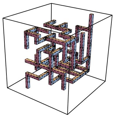
Visualize the boundary mesh with all boundaries grouped:

groups = bmesh["BoundaryElementMarkerUnion"];
temp = Most[Range[0, 1, 1/(Length[groups])]];
colors = ColorData["BrightBands"][#] & /@ temp;
bmesh["Wireframe"[
  "MeshElementStyle" -> (Directive[{FaceForm[#], EdgeForm[]}] & /@ 
     colors), PlotRange -> {{0, 5.4}, {0, 5.4}, {0, 5.4}}]]

enter image description here

You can then generate the full mesh:

AbsoluteTiming[mesh = ToElementMesh[bmesh]]
(* {22.961911`, 
 ElementMesh[{{0.5`, 5.5`}, {0.5`, 5.5`}, {0.5`, 
    5.5`}}, {TetrahedronElement["<" 963565 ">"]}]} *)
$\endgroup$

Your Answer

By clicking “Post Your Answer”, you agree to our terms of service and acknowledge you have read our privacy policy.

Not the answer you're looking for? Browse other questions tagged or ask your own question.