On random numbers extracted from NormalDistribution by two different methods under the same seed

Question

I've encountered the following situation within various trials.

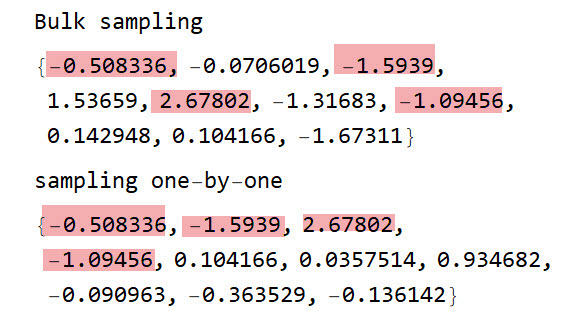
Why does such a difference arise between bulk sampling and one-by-one sampling?

(*Bulk sampling*)
SeedRandom[1234];
RandomVariate[NormalDistribution[], 10]

(*sampling one-by-one*)
SeedRandom[1234];
Table[RandomVariate[NormalDistribution[]], 10]

Example: For example, consider the following game.

• The player gains points depending on the value of variable x every time.
• x is a random number, and is subject to NormalDistribution [0, 1]
• If x> 0 then the player gets + 1,otherwise, x <0, the player gets -1.

I believed that expectation value of game scores should be equal regardless of how random numbers are generated.

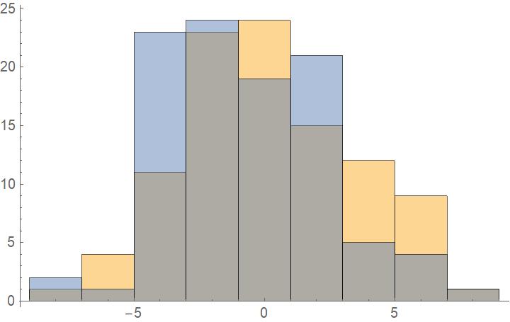
However, the experiment is as follows.
About Mean:

{BlockRandom[SeedRandom[1234]; 
  N@Mean@Table[
     Total[If[# > 0, 1, -1] & /@ 
       RandomVariate[NormalDistribution[], 10]], {100}]],
 BlockRandom[SeedRandom[1234]; 
  N@Mean@Table[
     Total[If[# > 0, 1, -1] & /@ 
       Table[First@RandomVariate[NormalDistribution[], 1], 
        10]], {100}]]}

{0.18, -0.68}

Histogram[{BlockRandom[SeedRandom[1234]; 
   Table[Total[
     If[# > 0, 1, -1] & /@ 
      RandomVariate[NormalDistribution[], 10]], {100}]],
  BlockRandom[SeedRandom[1234]; 
   Table[Total[
     If[# > 0, 1, -1] & /@ 
      Table[First@RandomVariate[NormalDistribution[], 1], 
       10]], {100}]]}]

I didn't understand why this happens and found out the phenomenon in this question.

Answer 1

I think this is due to the Box–Muller transform that is employed to generate pairs of normally distributed values. This method is much faster than using the inverse commulative probability function.

The algorithm is essentially as follows:

n = 1000000;
a = Flatten[ReIm[
   Times[
    Sqrt[-2. Log[RandomReal[{0, 1}, n]]],
    Exp[(2. Pi I) RandomReal[{0, 1}, n]]
    ]
   ]]; // AbsoluteTiming //First

0.003597

As comparison:

b = RandomVariate[NormalDistribution[], 2 n]; // AbsoluteTiming // First
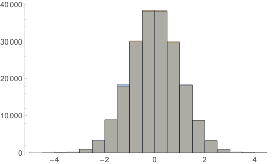
Histogram[{a, b}]

0.003579

Although I cannot reproduce the precise order used in Mathematica, the timings are very similar. I guess, this supports my hypothesis.

Whenever only a single sampling of the normal distribution is required, the second sampled value is just thrown away. This explains why the results of the bulk sampling equal the results one-by-one sampling, interleaved with other pseudorandom numbers.

Answer 2

When I change the distribution from NormalDistribution to UniformDistribution there is no difference in the two results.

SeedRandom[1234];
RandomVariate[UniformDistribution[], 10]

{0.876608, 0.521964, 0.0862234, 0.377913, 0.0116446, 0.927266, 0.543757, 0.479332, 0.245349, 0.759896}

SeedRandom[1234];
Table[First @ RandomVariate[UniformDistribution[], 1], 10]

{0.876608, 0.521964, 0.0862234, 0.377913, 0.0116446, 0.927266, 0.543757, 0.479332, 0.245349, 0.759896}

From this I conclude that the anomalous behavior is caused by the distribution function and not by RandomVariate. This is additional support for Henrik Schumacher's hypothesis.