Minimax optimization in Mathematica

Question

Mathematica has functions for constrained nonlinear maximization or minimization of functions, via FindMinimum and FindMaximum or similar functions.

I need to solve minimax problems of the form:

$$\min_x \max_y f(x,y)$$

subject to equality and inequality constrains of the form:

$$g_i(x) \le 0, \quad i = 1,\dots, p$$ $$h_j(y) \ge 0, \quad j = 1,\dots, q$$

$$A x + B y = c$$

Here $f(x,y)$ is convex in $x$ (for fixed $y$) and concave in $y$ (for fixed $x$). Moreover, $g_i(x)$ are convex, $h_j(y)$ concave, and $A,B$ matrices of appropriate dimensions.

Are there numerical algorithms in mathematica for these kinds of problems?

For example, Matlab offers the function fminimax.

Answer 1

According to the Matlab documentation:

fminimax minimizes the worst-case (largest) value of a set of multivariable functions, starting at an initial estimate. This is generally referred to as the minimax problem.

Doing this is straightforward in Mathematica, for example:

FindMinimum[{t, {t >= Sin[x], t >= Cos[x]}}, {t, x}]

finds the value of x such that Max[Sin[x],Cos[x]] is minimal.

The example from the Matlab documentation would be:

f[x_] := {
  2*x[[1]]^2 + x[[2]]^2 - 48*x[[1]] - 40*x[[2]] + 304,
  -x[[1]]^2 - 3*x[[2]]^2,
  x[[1]] + 3*x[[2]] - 18,
  -x[[1]] - x[[2]],
  x[[1]] + x[[2]] - 8
  }

FindMinimum[{t, Thread[t >= f[{x, y}]]}, {t, x, y}]

{1.71811*10^-7, {t -> 1.71811*10^-7, x -> 4., y -> 4.}}

which is the same solution Matlab gives. (The algorithm section says that fminmax does more or less the same thing)

---

If you want to solve a continous minimax problem, and yis only 1 or 2 variables, you can approximate it like this:

ys = Subdivide[-π, π, 100];
FindMinimum[{t, Thread[t >= Sin[x]*Sin[ys]]}, {t, x}]

Which is still surprisingly fast (0.03sec on my PC), but it doesn't scale if the domain of y is larger

Answer 2

There are also the undocumented, internal functions:

Optimization`FindMinimax
Optimization`FindMaximin
Optimization`NMinimax
Optimization`NMaximin

A typical call has the form

Optimization`FindMinimax[{f, cons}, vars, opts]

where f is a vector of objective functions. The call is translated to a call of the form

optimizer[{z, And @@ Flatten[{cons}, 1] && And @@ Thread[r[z, f]]}, vars, opts]

where optimizer is either FindMinimum, FindMaximum, NMinimize, or NMaximize, respectively. Essentially, then, this implements the same approach as @Niki.

@Niki's first example:

Optimization`FindMinimax[{{Sin[x], Cos[x]}, {}}, {x}]
(*  {0.707107, {x -> 0.785398}}  *)

My example doesn't give a good result, even with a pretty good starting point. It gives a minimum of 1344.09 with starting values of {{x, 5}, {y, 2}}. The "InteriorPoint" method gives a better result, a minimum of 43.1525 with automatically chosen starting points and good minimum with the starting point of {5, 2}:

Optimization`FindMinimax[{{Max[{Abs[2 x^2 + y^2 - 48 x - 40 y + 304], 
     Abs[-x^2 - 3 y^2], Abs[x + 3 y - 18], Abs[-x - y], 
     Abs[x + y - 8]}]},
  {}},
 {{x, 5}, {y, 2}}, Method -> "InteriorPoint"]
(*  {37.2375, {x -> 4.92671, y -> 2.07865}}  *)

Using the global optimizer NMinimize works a bit better:

Optimization`NMinimax[{{Max[{Abs[2 x^2 + y^2 - 48 x - 40 y + 304], 
     Abs[-x^2 - 3 y^2], Abs[x + 3 y - 18], Abs[-x - y], 
     Abs[x + y - 8]}]},
  {}},
 {x, y}]
(*  {37.239, {x -> 4.92601, y -> 2.07954}}  *)

The method "DifferentialEvolution" is slightly faster (1.35 sec. vs. 1.6 sec):

Optimization`NMinimax[{{Max[{Abs[2 x^2 + y^2 - 48 x - 40 y + 304], 
     Abs[-x^2 - 3 y^2], Abs[x + 3 y - 18], Abs[-x - y], 
     Abs[x + y - 8]}]},
  {}},
 {x, y},
 Method -> "DifferentialEvolution"]
(*  {37.239, {x -> 4.92601, y -> 2.07954}}  *)

Answer 3

From this tutorial:

(*FindMinMax[{Max[{f1,f2,..}],constraints},vars]*)
SetAttributes[FindMinMax, HoldAll];
FindMinMax[{f_Max, cons_}, vars_, opts___?OptionQ] := 
  With[{res = iFindMinMax[{f, cons}, vars, opts]}, 
   res /; ListQ[res]];
iFindMinMax[{ff_Max, cons_}, vars_, opts___?OptionQ] := 
  Module[{z, res, f = List @@ ff},
      res = FindMinimum[{z, (And @@ cons) && (And @@ Thread[z >= f])}, 
     Append[Flatten[{vars}, 1], z], opts]; 
   If[ListQ[res], {z /. res[[2]], 
     Thread[vars -> (vars /. res[[2]])]}]];

An example:

FindMinMax[{Max[{Abs[2 x^2 + y^2 - 48 x - 40 y + 304], 
    Abs[-x^2 - 3 y^2], Abs[x + 3 y - 18], Abs[-x - y], 
    Abs[ x + y - 8]}], {}}, {x, y}]

(*  {37.2356, {x -> 4.92563, y -> 2.07956}}  *)

A few more examples are in the tutorial.

Answer 4

You could split your problem:

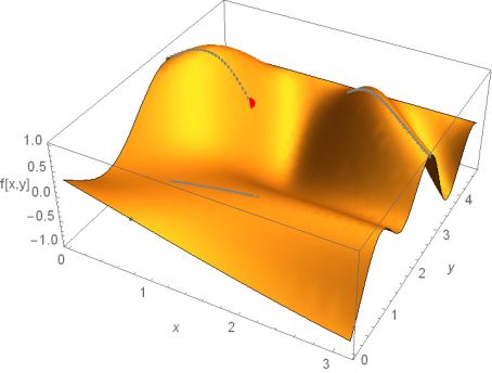
As an example I consider the function

f[x_, y_] := Sin[(x - Pi/4) ( y - Pi/8)] Cos[y]

First step looks for maxima y[x]

maxy[x_?NumericQ] := y /. NMaximize[ {f[x, y], 0 <= y <= 3/2 Pi}, y][[2]]

Among all these points {x,maxy[x],f[x,maxy[x]]} the minimum is evaluated:

min = NMinimize[{f[x, maxy[x]] , 0 <= x <= Pi}, x ]
(* takes some time...*)

and plotted (red point is the minmax!)

minP = {x /. #[[2]], maxy[x /. #[[2]]], #[[1]]} &[min];
(*{0.785398, 3.45703, 9.78576*10^-11}*)
Show[{Plot3D[ f[x, y], {x, 0, Pi}, {y, 0,  3/2 Pi}, Mesh -> False,AxesLabel -> {x, y, f}],Graphics3D [{Gray, 
Point[Table[{x, maxy[x], f[x, maxy[x]]}, {x, 0, Pi, Pi/100}]], 
Red, PointSize[.025], Point[minP]}] }, AxesLabel -> {x, y, "f[x,y]"}]