Introduction
I would have done a Chebyshev approach earlier, but a stupid, elusive typo kept the accuracy low. The method is fast and highly accurate, although for the code below, recursive refinement and a convergence test have not been implemented (the idea would be the same as used for cheb`approx in this answer).
A discussion of this approach, as well as an example over an infinite interval, may be found in this answer. Here we need only a simple affine transformation of a finite interval to the standard Chebyshev interval $[-1, 1]$. See Boyd, Chebyshev and Fourier Spectral Methods (2001) for more.
OP's problem
For convenience, here is the OP's setup:
eps = 1/100;
eq = (eps^2) y''[x] + eps*x*y'[x] - y[x] == -Exp[x];
bcs = {y[0] == 2, y[1] == 1};
Chebyshev series solutions of linear, second-order BVPs
First we give a general function that will solve a linear, second-order BVP. It depends on some utilities given at the end.
ClearAll[chebLinearSecondOrderBVP, chebLinearSecondOrderBVP`parse];
Options[chebLinearSecondOrderBVP] = {WorkingPrecision -> MachinePrecision};
SetAttributes[chebLinearSecondOrderBVP`parse, HoldAllComplete];
(* parses the input; TBD: error messages! *)
chebLinearSecondOrderBVP`parse[
   chebLinearSecondOrderBVP[sys_, y_, {x_, a_?NumericQ, b_?NumericQ},
    n_, opts : OptionsPattern[chebLinearSecondOrderBVP]]] :=
  Module[{ode, bcs, odebcs, dorder, y1, y2, prec},
   With[{f = FreeQ[#, y[x] | Derivative[_][y][x]] &},
    odebcs = SortBy[f]@GatherBy[sys, f]
    ];
   If[Length /@ odebcs == {1, 2},
    {{ode}, bcs} = odebcs,
    Return[$Failed]];
   {y1, y2} = {y[a], y[b]} /. First@Solve[bcs, {y[a], y[b]}];
   If[! VectorQ[{y1, y2}, NumericQ], Return[$Failed]];
   dorder = Max@Cases[ode, Derivative[k_][y][x] :> k, Infinity];
   If[dorder != 2, Return[$Failed]];
   If[! Internal`LinearQ[ode, {y[x], y'[x], y''[x]}], Return[$Failed]];
   prec = OptionValue[chebLinearSecondOrderBVP, opts, WorkingPrecision];
   {ode, y1, y2, prec}
   ];
call : chebLinearSecondOrderBVP[
    sys_, y_, {x_, a_?NumericQ, b_?NumericQ}, n_, OptionsPattern[]] :=
  Module[{ode, y1, y2, xvec, dm, dops, opL, load, dy, yvec, cc, prec, res},
   res = chebLinearSecondOrderBVP`parse[call]; (* parse arguments *)
   (
     {ode, y1, y2, prec} = res;
     (* construct differential operator  opL  for the ode *)
     ode = Normal@ CoefficientArrays[ode /. Equal -> Subtract, {y[x], y'[x], y''[x]}];
     {dm, {{xvec}}} = Reap[chebDM[n, prec], "x"];  (* Ch. deriv. operator and pts. *)
     dops = NestList[2/(b - a) dm.# &, IdentityMatrix[n + 1], 2]; (* 0-2 order diff.ops.*)
     dops = dops[[All, 2 ;; -2, 2 ;; -2]];         (* strip boundary *)
     xvec = Rescale[xvec[[2 ;; -2]], {-1, 1}, {a, b}];
     opL = (ode[[2]] /. x -> xvec) dops // Total;  (* assumes coefficients are Listable *)
     (* construct load and subtract line to make homogeneous BCs y[a]==y[b]==0:
      * the line affects the y[x], y'[x] terms (ode[[2,1;;2]]);
      * it does not affect the y''[x] term
      *)
     load = ode[[1]] /. x -> xvec;
     dy = {(a y2 - b y1 + x (y1 - y2))/(a - b), (y2 - y1)/(b - a)} ode[[2, 1 ;; 2]] /.
        x -> xvec // Total;                        (* impose homogeneous BCs *)
     (* solve BVP, get Chebyshev coeffs and add line back for BVs *)
     yvec = LinearSolve[opL, -load - dy];
     yvec = ArrayPad[yvec, 1, N[0, prec]];         (* added homogenized BCs *)
     cc = chebSeries[yvec];
     cc[[1]] += (y1 + y2)/2;  (* Adjust to BCs *)
     cc[[2]] += (y2 - y1)/2;
     res = chebFunc[cc, {a, b}]
     ) /; FreeQ[res, $Failed | chebLinearSecondOrderBVP`parse]
   ];
The solution of the OP's problem:
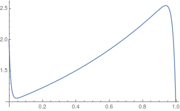
ySol2 = chebLinearSecondOrderBVP[{eq, y[0] == 2, y[1] == 1},
   y, {x, 0, 1}, 64, WorkingPrecision -> 32];

Plot[{Exp[x], ySol2[x]}, {x, 0, 1}]
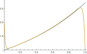
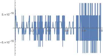
The solution satisfies the BVP to machine precision
Plot[Evaluate[eq /. Equal -> Subtract /. y -> ySol2], {x, 0, 1},
 PlotRange -> All, PlotPoints -> 200]
{y[0.] - 2, y[1.] - 1} /. y -> ySol2  (* BCs *)
(*  {0., 0.}  *)
Chebyshev utilities
(*
 * Chebyshev series utilities
 *)

ClearAll[chebFunc];
chebFunc::usage = "f = chebFunc[c,{a,b}], c = {c0, c1,..., cn} Chebyshev coefficients, over the interval {a,b}; y = chebFunc[c,{a,b}][x] evaluates the function";
chebFunc[c_, {a_, b_}][x_] := chebFunc[c, {a, b}, x];
chebFunc[c_?(VectorQ[#, NumericQ] &), {a_?NumericQ, b_?NumericQ}, x_?NumericQ] :=
  ChebyshevT[Range[0, Length[c] - 1], (2 x - (a + b))/(b - a)].c;
chebFunc[c_?(VectorQ[#, NumericQ] &), {a_?NumericQ, b_?NumericQ}, x_?(VectorQ[#, NumericQ] &)] :=
  Cos[Outer[Times, ArcCos[(2 x - (a + b))/(b - a)], Range[0, Length[c] - 1]]].c;
chebFunc /: Normal[chebFunc[c_?VectorQ, {a_, b_}, x_]] :=
  Evaluate@ChebyshevT[#, (2 x - (a + b))/(b - a)] &[Range[0, Length[c] - 1]].c;
Derivative[_, _, n_][chebFunc][c_, {a_, b_}, x_] /; 0 <= n <= Length@c :=
  chebFunc[Nest[chebDerivative, c, n] (2/(b - a))^n, {a, b}, x];

ClearAll[chebDerivative, chebSeries, chebDM];
chebDerivative::usage = "chebDerivative[c, {a,b}] differentiates the Chebyshev series c scaled over the interval {a,b}";
chebDerivative[c_] := chebDerivative[c, {-1, 1}];
chebDerivative[c_, {a_, b_}] :=
  Module[{c1 = 0, c2 = 0, c3},
   2/(b - a) MapAt[#/2 &,
     Reverse@Table[
       c3 = c2;
       c2 = c1;
       c1 = 2 (n + 1)*c[[n + 2]] + c3,
       {n, Length[c] - 2, 0, -1}],
     1]];
chebDM::usage = "chebD[n] = (n+1)x(n+1) Chebyshev spectral differentiation matrix of order n";
chebDM[n_Integer?Positive, prec_ : MachinePrecision] :=
 Module[{fac, xm},
  xm = If[prec === MachinePrecision,
    ConstantArray[Sin[(π Range[N[n], -N[n], -2.])/(2 n)], n + 1],
    ConstantArray[N[Sin[(π Range[n, -n, -2])/(2 n)], prec], n + 1]];
  Sow[First[xm], "x"];
  fac = Flatten[{2, PadRight[{}, n - 1, {-1, 1}], 2 - 4 Mod[n, 2]}];
  xm = Outer[Times, fac, 1/fac]/(Transpose[xm] - xm + IdentityMatrix[n + 1]);
  xm - DiagonalMatrix[Total[xm, {2}]]];

chebSeries::usage = "chebSeries[y] returns the Chebyshev series for the function values y over the standard interval {-1, 1}";
chebSeries[y_] := Module[{cc},
   cc = Sqrt[2/(Length[y] - 1)] FourierDCT[y, 1];
   cc[[{1, -1}]] /= 2;
   cc];


y[x] == Exp[x], which itself does not satisfy the BCs. It's not surprising it's ill-conditioned. It's probably unstable asepsgoes to zero. I suppose this is what you're studying? $\endgroup$