NDSolve: multi-dimensional, variable boundary condition

Question

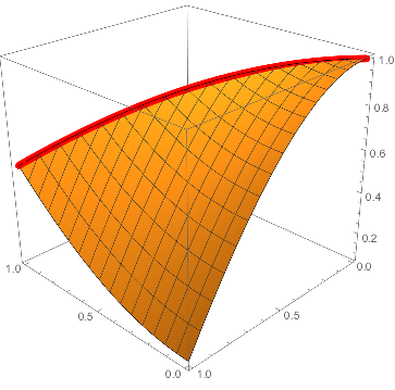
For a simplified 2D system, consider the case where the boundary condition for a differential equation that lies on a line in the $x,y$ plane: for example, I know the value of $\partial_x f[x,y]$ for all $x,y$ and the value of $f[x,x]$ for any $x$ which is used as my boundary condition (the boundary condition is here given on a 45 degree line in the x-y plane, and not, say at $x=0$). My attempts at using NDSolve[] to deal with this is not successful. For example,

NDSolve[{D[f[x, y], x] == Sin[x], f[a, a] == Cos[a]}, f, {x, 0, 1}, {y, 0, 1}]

gives

NDSolve::litarg: To avoid possible ambiguity, the arguments of the dependent variable in f[a,a]==Cos[a] should literally match the independent variables.

And writing the boundary condition as f[x,x]==Cos[x] gives NDSolve::conarg: The arguments should be ordered consistently.

Another attempt I've tried is using DirichletCondition, e.g.

r = ImplicitRegion[x <= y && x >= 0 && y >= 0 && x <= 1 && y <= 1, {x, y}]
sol = NDSolveValue[{D[f[x, y], x] == Sin[x], DirichletCondition[f[x, y] == Cos[x], x == y]}, f, {x, y} \[Element] r]

but that gives NDSolveValue::femcscd: The PDE is convection dominated and the result may not be stable. Adding artificial diffusion may help. While the result given appears reasonable with this simplified model(red line=boundary condition),

Show[{ParametricPlot3D[{x, x, Cos[x]}, {x, 0, 1}, 
   PlotStyle -> {Red, Thickness[.02]}], 
  Plot3D[sol[x, y], {x, y} \[Element] r]}, PlotRange -> All]

I'm worried about the applicability of this for my complex system (e.g. thousands runs with random parameters in the equation, not practical to check each run). I could manually integrate the equation inside a loop, choosing some appropriate step length, but I want to learn how to employ NDSolve directly to get a numerical solution to the equation.

Answer 1

We can do this analytically.

pde = D[f[x, y], x] == Sin[x];

Integrate[pde[[1]], x] == Integrate[pde[[2]], x] + g[y]
(*f[x, y] == g[y] - Cos[x]*)

Added the arbitrary function g[y]. Now apply your bc

% /. {y -> x};

g[x_] = g[x] /. Solve[(% /. f[x, x] -> Cos[x]), g[x]][[1]]
(*2 Cos[x]*)

f[x_, y_] = int[[2]]
(*2 Cos[y] - Cos[x]*)

pde
(*True*)

f[x, x]
(*Cos[x]*)

f[a, a]
(*Cos[a]*)

Update

NDSolve will solve the bc f[a,a]==Cos[a] if you define a numerically and:

Clear[f]

pde = D[f[x, y], x] == Sin[x]

a = .5;

sol1 = NDSolve[{pde, f[a, y] == Cos[y]}, f, {x, 0, 1}, {y, 0, 1}] // Flatten;

{(f[a, a] /. sol1), Cos[a]}
(*{0.877583,0.877583}*)

Evidently NDSolve has trouble if there is no information on y at all as in f[x,x] == Cos[x] and unfortunately f[a,a] only matches f[x,x] at one point.