Findroot with a precompiled function with parameters

Question

If I want to precompile a function that I intend to put into FindRoot many times, I could do it like this:

f[x_] := x^x + (4 - x)^(4 - x) - 10
g = Compile[{x}, Evaluate[f[x]]];
FindRoot[g, {3.99}]

Then if I want to run FindRoot on this function multiple times it will be faster. Generally FindRoot will compile the input function as the function will be called many times, and now if I want to run FindRoot itself many times (for example with different initial conditions to find different roots of the function) the function is compiled only once.

Now suppose that I have a similar function which depends also on a parameter. I'd like to be able to compile the function only once (and not for every value of a), and use FindRoot for different values of the parameter like so:

f[x_, a_] := x^x + (a - x)^(a - x) - 10
FindRoot[f[x, 4], {x, 3.99}]
FindRoot[f[x, 5], {x, 4.99}]

I can't work out I would do this, can anybody help?

Answer 1

In order to profit from compilation, you have to ensure that f gets really compiled. With can help here. In order to allow for Newton's method, we compile the expression for f and its derivative with respect its first argument into CompiledFunctions cf and cDf that expect vector-valued input.

f[x_, a_] := x^x + (a - x)^(a - x) - 10;
Quiet[Block[{x, a},
   cf = With[{code = N[{f[x[[1]], a[[1]]]}]},
     Compile[{{x, _Real, 1}, {a, _Real, 1}}, code]
     ];
   cDf = With[{code = N[D[{f[x[[1]], a[[1]]]}, {{x[[1]]}, 1}]]},
     Compile[{{x, _Real, 1}, {a, _Real, 1}}, code]
     ];
   ]
  ];

We use wrappers F and DF that only evaluate if vector-valued arguments are supplied in order to hand them over to FindRoot. Note the many braces for the initial value.

F[a_] := With[{ccf = cf}, x \[Function] ccf[x, a]];
DF[a_] := With[{ccDf = cDf}, x \[Function] (ccDf[x, a])];
FindRoot[F[{4.}], {{{3.99}}}, Jacobian -> DF[{4.}]]

{{2.37473}}

Answer 2

I know the specific question is about using a compiled function in FindRoot, but I would like to point out that sometimes compiled functions are slower than the vectorized/auto-parallelized functions in the MKL (on Intel machines) that underlie basic mathematical functions, such as those found in polynomials, in which the OP expressed interest in a comment.

Below is a vectorized FindRoot for solving 100,000 problems of the type in the question. It takes a little over a half second on average. On my machine it uses all cores fully while computing (I have 4, 8 virtual, and the CPU runs at 400%).

ClearAll[f];
f[x_?VectorQ, a_?VectorQ] := x^x + (a - x)^(a - x) - 20;
df0[x_?VectorQ, a_?VectorQ] = D[x^x + (a - x)^(a - x) - 20, x];
df[x_?VectorQ, a_?VectorQ] := DiagonalMatrix@SparseArray@df0[x, a];
params = RandomReal[{3, 5}, 100000];
FindRoot[f[x, params], {x, 2 params/3}, Jacobian :> df[x, params]]; // RepeatedTiming

(*  {0.539, Null}  *)

By comparison, running FindRoot on the OP's nonparametric example 100,000 times takes over 35 seconds. (Even if I use ParallelDo, it takes 8.5 sec., more than 10 times slower.)

ClearAll[f];
f[x_] := x^x + (4 - x)^(4 - x) - 10
g = Compile[{x}, Evaluate[f[x]]];
Do[FindRoot[g, {3.99}], {100000}]; // AbsoluteTiming

(*  {35.7169, Null}  *)

It is hard to be sure from the comment whether such an approach could be adapted to the OP's actual use-case, but it works quite well on the problem described in this question.

Answer 3

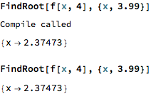
A simple idiom to do this is the following:

Module[{fc},
 fc[a_] := fc[a] = (Print["Compile called"]; Compile[{x}, x^x + (a - x)^(a - x) - 10]);
  f[x_?NumericQ, a_?NumericQ] := fc[a][x];
 ]

The trick is that when f is called, it calls fc[a] which compiles the function for a specific a and stores it through Memoization. After this first call, it will use the stored compiled function.

Therefore, compile is called only once for each different a.

Edit

Obviously, I misunderstood the question.

I want to compile only once for all values of a. This was what I meant in my wording of the original question, but I have edited to be more clear.

However, I don't see why you don't simply use

fc = Compile[{x, a}, x^x + (a - x)^(a - x) - 10];
f[x_?NumericQ, a_?NumericQ] := fc[x, a];

It should be noted that your original code

f[x_] := x^x + (4 - x)^(4 - x) - 10
g = Compile[{x}, f[x]];

doesn't do much good. f is not compiled. Instead, you are making the situation worse by creating a compiled function that calls back to the main kernel. Please use <<CompiledFunctionTools` and CompilePrint[g] to see your compiled code. Your expression is not included.

Another thing is that the more general expression with a will become complex for certain points and Mathematica will warn you about this.

Answer 4

Instead of using FindRoot with a parameter, you could use NDSolve. For your example this would be:

f[x_, a_] := x^x + (a-x)^(a-x) - 10

(* initial value *) 
x4 = x /. FindRoot[f[x, 4] == 0, {x, 3.99}]

(* ode *)
eqn = D[f[x[a], a], a] == 0

(* NDSolveValue *)
sol = NDSolveValue[{eqn, x[4] == x4}, x, {a, 2, 10}]

2.37473

(a - x[a])^( a - x[a]) (1 + Log[a - x[a]] (1 - Derivative1[x][a]) - Derivative1[x][a]) + x[a]^x[a] (Derivative1[x][a] + Log[x[a]] Derivative1[x][a]) == 0

NDSolveValue::mxst: Maximum number of 51511 steps reached at the point a == 2.450725468002232`.

NDSolveValue::ndsz: At a == 4.258744344333925`, step size is effectively zero; singularity or stiff system suspected.

InterpolatingFunction[{{2.45073, 4.25874}}, <>]

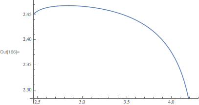
And a plot:

Plot[sol[a], {a, Sequence@@sol["Domain"][[1]]}]