Derivative of an interpolated function on an unstructured grid

Question

I'm writing my own FEM Poisson equation solver in C++ and I'm using Mathematica as a benchmark - currently it seems that my program outputs a correct solution, however I want to check whether the laplacian of the result is equal to the right-hand side. Unfortunately, the interpolation itself raises a warning "Interpolation on unstructured grids is currently only supported for InterpolationOrder->1 or InterpolationOrder->All. Order will be reduced to 1". FEM deals with mostly unstructured grids, so as a result, the order of interpolation is now 1 (piecewise linear functions). It is no surprise that when I try to compute the laplacian of the result, I get flat zero function.

For the sake of simplicty, let's use the following code

ClearAll[x, y]
c = {}; n = 10000;
For[i = 0, i <= n, i++,
 p = {x -> Random[], y -> Random[]};
 AppendTo[c, {x, y, Sin[5 x] Sinh[5 y] + 1/6 x^3 - 1/12 y^4} /. p];
 ]

The following

f = Interpolation@c;
lapf = D[f[x, y], {x, 2}] + D[f[x, y], {y, 2}];
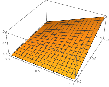
Plot3D[lapf, {x, 0, 1}, {y, 0, 1}]

gives flat zero function, although the laplacian of Sin[5 x] Sinh[5 y] + 1/6 x^3 - 1/12 y^4 is x - y^2. What can be done in case I have only numerical data on an unstructured grid and I need to evaluate laplacian at some point?

Answer 1

You could import your higher order mesh (2nd order is possible) and construct an ElementMesh from the data like so:

Needs["NDSolve`FEM`"]
mesh = ToElementMesh[
   "Coordinates" -> {{0., 0.}, {1., 0.}, {1., 1.}, {0., 1.}, {0.5, 
      0.}, {1., 0.5}, {0.5, 0.5}, {0.5, 1.}, {0., 0.5}}, 
   "MeshElements" -> {TriangleElement[{{1, 2, 3, 5, 6, 7}, {3, 4, 1, 
        8, 9, 7}}]}];

Construct some example values.

values = Function[{x, y}, x*y] @@@ mesh["Coordinates"];

Create the interpolating function.

if = ElementMeshInterpolation[{mesh}, values];

Plot the result.

Plot3D[if[x, y], {x, y} \[Element] mesh]

However, be careful with computing second order derivatives for that; this is more of a test of the interpolating function that it is for the PDE solver you write.

To test the solver you use an somewhat arbitrary expression and insert that in the differential equation. That will give you a right hand side. Solve the PDE with this new right hand side and check how close the solution is to the somewhat arbitrary expression you used to create the right hand side. This process is called manufactured solution.

Answer 2

First, instead of procedural code to produce your sample data, how about using functional programming on a smaller sample of 200 points:

data = Apply[
  Function[{x, y}, 
    {x, y, Sin[5 x] Sinh[5 y] + (1/6) x^3 - (1/12) y^4}
  ], RandomReal[{0, 1}, {200, 2}], 1]

Then, as the warning message suggests, try

f = Interpolation[data, InterpolationOrder -> All]

A plot of f shows that it agrees well with your original function. Next compute the Laplacian

lapf = Function[{x, y}, Evaluate[Laplacian[f[x, y], {x, y}]]]

which also agrees very well with the Laplacian of f.