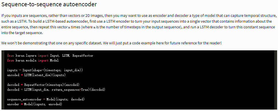
According Keras blog,I find the Seq2Seq auto-encoder. But it didn't give any example only code.
To build a LSTM-based autoencoder, first use a LSTM encoder to turn your input sequences into a single vector that contains information about the entire sequence, then repeat this vector n times (where n is the number of timesteps in the output sequence), and run a LSTM decoder to turn this constant sequence into the target sequence.
So I try to make similar thing in Mathematica using MNIST database.
resource = ResourceObject["MNIST"];
trainingData = ResourceData[resource, "TrainingData"];
testData = ResourceData[resource, "TestData"];
trainingSubset = Select[trainingData, Last[#] <= 4 &];
testSubset = Select[testData, Last[#] <= 4 &];
trainingImages = Keys[trainingSubset];
meanImage = Image[Mean@Map[ImageData, trainingImages]];
This is normal DNN auto-encoder of MNIST.
encoder = NetChain[{FlattenLayer[], 100, Ramp, 50, Ramp, 16}];
decoder = NetChain[{32, 50, Ramp, 100, Ramp, 784, ReshapeLayer[{1, 28, 28}]}];
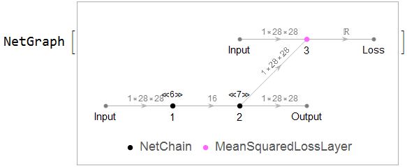
net = NetGraph[{encoder, decoder, MeanSquaredLossLayer[]}, {1 -> 2 -> NetPort["Output"], 2 -> NetPort[3, "Input"], NetPort["Input"] -> NetPort[3, "Target"]},
               "Input" -> NetEncoder[{"Image", {28, 28}, "Grayscale", "MeanImage" -> meanImage}],
               "Output" -> NetDecoder[{"Image", "Grayscale"}]]
{lossplot1, trained} = NetTrain[net, <|"Input" -> trainingImages|>, "Loss",
                                {"LossEvolutionPlot", "TrainedNet"},
                                BatchSize -> 256, MaxTrainingRounds -> 10];
We could explore the visulization of it.
reconstructor = Take[trained, {NetPort["Input"], NetPort["Output"]}];
BlockRandom[
 Grid[{#, ImageAdd[reconstructor[#], meanImage] & /@ #} &@
   RandomSample[trainingImages, 10]], RandomSeeding -> 1234]
encoder = Take[trained, {NetPort["Input"], 1}];
testImages = Keys[testSubset];
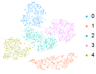
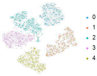
coords = DimensionReduce[encoder[testImages], 2, Method -> "TSNE"];
labels = Values[testSubset];
ListPlot[Table[Extract[coords, Position[labels, i]], {i, 0, 4}],
 PlotLegends -> PointLegend[96, Range[0, 4]], Axes -> None,
 PlotStyle -> Map[ColorData[96], Range[1, 5]], AspectRatio -> 1,
 ImageSize -> Small]
But using autoencoder based LSTM,the result isn't good.
encoder = NetChain[{ReshapeLayer[{28, 28}], LongShortTermMemoryLayer[16],
                    SequenceLastLayer[]}];
decoder = NetChain[{ReplicateLayer[28], LongShortTermMemoryLayer[28],
                    ReshapeLayer[{1, 28, 28}]}];
net = NetGraph[{encoder, decoder, MeanSquaredLossLayer[]}, {1 -> 2 -> NetPort["Output"], 2 -> NetPort[3, "Input"], NetPort["Input"] -> NetPort[3, "Target"]},
                "Input" -> NetEncoder[{"Image", {28, 28}, "Grayscale", "MeanImage" -> meanImage}],
                "Output" -> NetDecoder[{"Image", "Grayscale"}]]
{lossplot2, trained} = NetTrain[net, <|"Input" -> trainingImages|>, "Loss",
                                {"LossEvolutionPlot", "TrainedNet"},
                                BatchSize -> 256, MaxTrainingRounds -> 10];
reconstructor = Take[trained, {NetPort["Input"], NetPort["Output"]}];
BlockRandom[Grid[{#, ImageAdd[reconstructor[#], meanImage] & /@ #} &@
   RandomSample[trainingImages, 10]], RandomSeeding -> 1234]
encoder = Take[trained, {NetPort["Input"], 1}];
testImages = Keys[testSubset];
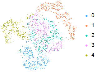
coords = DimensionReduce[encoder[testImages], 2, Method -> "TSNE"];
labels = Values[testSubset];
ListPlot[Table[Extract[coords, Position[labels, i]], {i, 0, 4}],
 PlotLegends -> PointLegend[96, Range[0, 4]], Axes -> None,
 PlotStyle -> Map[ColorData[96], Range[1, 5]], AspectRatio -> 1,
 ImageSize -> Small]
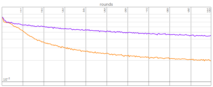
The loss of LSTM(purple color) fall down slowly
Show[{lossplot1, lossplot2 /. Hue[__] -> Hue[0.75]}]
How to improve the result?
PS:Using LSTM to predict digits number in MNIST got a good result even data is image instead of temporal time-series in this case
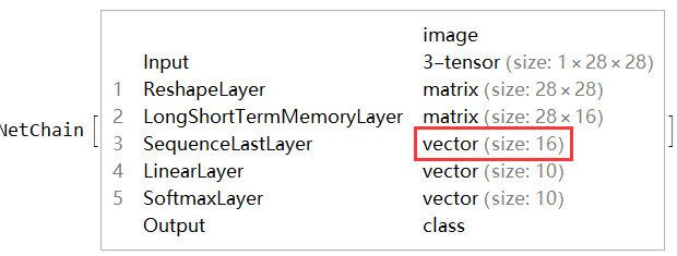
Using LSTM,the dimensions of embedding vector after LSTM is also 16,it can be think a presentation or encoder of the image.
why in the above case,same embedding vector size can't get a pretty good result of auto-encoder?
lstmnet = NetChain[{ReshapeLayer[{28, 28}], LongShortTermMemoryLayer[16],
                    SequenceLastLayer[], LinearLayer[5], SoftmaxLayer[]},
                    "Output" -> NetDecoder[{"Class", Range[0, 4]}],
                    "Input" -> NetEncoder[{"Image", {28, 28}, "Grayscale"}]];
trained = NetTrain[lstmnet, trainingSubset, ValidationSet -> testSubset,
                   BatchSize -> 256, MaxTrainingRounds -> 5]
ClassifierMeasurements[trained, testSubset]["Accuracy"]
(*0.965947*)
Using CNN(lenet version)
lenet = NetChain[{ConvolutionLayer[20, 5], Ramp, PoolingLayer[2, 2],
                  ConvolutionLayer[50, 5], Ramp, PoolingLayer[2, 2], FlattenLayer[],
                  500, Ramp, 5, SoftmaxLayer[]},
                  "Output" -> NetDecoder[{"Class", Range[0, 4]}],
                  "Input" -> NetEncoder[{"Image", {28, 28}, "Grayscale"}]];
trained = NetTrain[lenet, trainingSubset, ValidationSet -> testSubset,
                   BatchSize -> 256,MaxTrainingRounds -> 5]
ClassifierMeasurements[trained, testSubset]["Accuracy"]
(*0.997081*)

