4
$\begingroup$

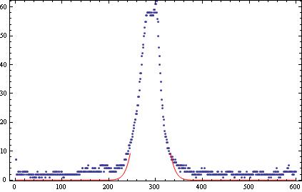
I have some data and want to fit it with a Gaussian distribution. The problem is that Mathematica only fits it partly. I have tried to write the code in three different ways, but none of them worked.

First method

dat = ImportString[Import["PirmaisPikis.txt"], "Table"];
Gauss[A_, σ_, μ_, x_] := (A*1)/(σ*(2*π)^(0.5))*
  Exp[(-0.5)*((x - μ)/σ)^2]
fit = NonlinearModelFit[dat, 
  Gauss[A, σ, μ, 
   x], {{σ, 22}, { μ, 300}, {A, 3360}}, x]
Show[ListPlot[dat2], Plot[fit[ x], {x, 0, 600}, PlotStyle -> Red] , 
 PlotRange -> {All, All}, Frame -> True]

enter image description here

Second method

dat = ImportString[Import["PirmaisPikis.txt"], "Table"];
Gauss[A_, σ_, μ_, x_] := (A*1)/(σ*(2*π)^(0.5))*
  Exp[(-0.5)*((x - μ)/σ)^2]
fittesana = 
 FindFit[dat, Gauss[A, σ, μ, x], {σ, μ, A}, x]
Show[ListPlot[dat2], Plot[fit[ x], {x, 0, 600}] , 
 PlotRange -> {All, All}, Frame -> True]
{σ -> 22.2196, μ -> 288.645, A -> 3355.57} (and picture shown before)

Third method

dat = ImportString[Import["PirmaisPikis.txt"], "Table"];
Gauss[A_, σ_, μ_, x_] := (A*1)/(σ*(2*π)^(0.5))*
  Exp[(-0.5)*((x - μ)/σ)^2]
fittesana = 
 FindFit[dat, 
  Gauss[A, σ, μ, x], {20 < σ < 22, 
   200 < μ < 300, 3300 < A < 3400}, x]
Show[ListPlot[dat2], Plot[fit[ x], {x, 0, 600}] , 
 PlotRange -> {All, All}, Frame -> True]

FindFit::fdssnv: Search specification 20<σ<22 without variables should be a list with 1 to 4 elements. >>

Link to PirmaisPikis.txt

What is my problem?

$\endgroup$

2 Answers 2

9
$\begingroup$

It is simply a plotting problem.

As a side note, you can import the data directly from the web using

dat = Import["https://pastebin.com/raw/w9ys8Rfd", "Table"];

Then your code:

Gauss[A_, σ_, μ_, x_] := (A*1)/(σ*(2*π)^(0.5))*Exp[(-0.5)*((x - μ)/σ)^2]
fit = NonlinearModelFit[dat, 
  Gauss[A, σ, μ, x], {{σ, 22}, { μ, 300}, {A, 3360}}, x];

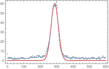
Here we come to the problem. In Show, you are combining two plots. The second one is plotted in Automatic and clips the top part (missing red curve). Simply add option PlotRange -> Full in Plot, such as in:

Show[Plot[fit[x], {x, 0, 600}, PlotStyle -> Red, PlotRange -> Full], 
 ListPlot[dat], Frame -> True]

enter image description here

$\endgroup$
6
$\begingroup$

It would be helpful if you mention something about the source and structure of the data. For example, the "y" values are all integers. Are these frequency counts? Or are they discrete measurements at each of the 600 "x" values?

If the "y" values are frequencies and you are trying to fit a normal distribution, then all you need to do is find the mean and standard deviation of the data. (However, you definitely don't have samples from a normal distribution. Maybe samples from a normal distribution contaminated with a discrete uniform distribution.)

If the "y" values are measurements, then you want to perform a regression (rather than fitting a probability distribution with implied sampling properties) that just happens to have a similar shape to a normal probability density function.

A curve following a normal probability function will drop to zero quickly and your data does not support that. What you can do is add another parameter that raises the curve a bit to get a more appropriate regression fit. I've added the parameter a0 below to raise the curve and obtain a better fit.

Below I've re-parameterized such a curve to avoid any hint that there might be random sampling properties implied (i.e., no mean and standard deviation) under the assumption that this is a regression problem.

y = {7, 7, 2, 2, 2, 3, 2, 3, 2, 2, 3, 2, 2, 2, 3, 2, 3, 3, 2, 3, 3, 3,
    2, 3, 3, 3, 2, 2, 2, 2, 2, 1, 2, 2, 2, 2, 1, 2, 2, 1, 1, 1, 2, 1, 
   2, 2, 3, 2, 2, 1, 2, 1, 2, 2, 2, 2, 1, 2, 2, 2, 2, 2, 2, 2, 1, 3, 
   2, 2, 2, 2, 2, 2, 1, 2, 2, 2, 2, 2, 2, 2, 3, 2, 2, 3, 3, 2, 2, 3, 
   3, 2, 2, 2, 3, 3, 2, 2, 2, 3, 3, 2, 2, 2, 1, 1, 2, 2, 2, 2, 2, 2, 
   2, 2, 2, 2, 2, 2, 2, 2, 2, 2, 2, 2, 2, 2, 2, 2, 2, 2, 2, 2, 2, 2, 
   3, 2, 3, 3, 2, 3, 3, 3, 3, 3, 4, 4, 3, 3, 3, 3, 3, 4, 3, 4, 4, 4, 
   3, 5, 3, 3, 3, 3, 3, 3, 3, 3, 4, 3, 4, 3, 4, 3, 4, 3, 3, 3, 3, 3, 
   3, 4, 3, 3, 3, 5, 5, 3, 5, 5, 5, 5, 5, 3, 4, 5, 5, 4, 5, 4, 5, 4, 
   4, 4, 3, 4, 3, 3, 4, 3, 3, 3, 3, 3, 3, 4, 3, 3, 4, 3, 5, 4, 5, 4, 
   5, 4, 4, 5, 5, 5, 5, 4, 5, 5, 5, 5, 7, 7, 7, 7, 9, 9, 9, 9, 9, 10, 
   12, 11, 12, 13, 13, 14, 14, 15, 16, 17, 18, 19, 20, 21, 21, 23, 23,
    24, 26, 26, 29, 29, 31, 34, 35, 37, 37, 40, 43, 44, 46, 47, 50, 
   51, 53, 55, 55, 57, 57, 58, 58, 58, 58, 58, 58, 58, 57, 57, 57, 58,
    57, 57, 57, 58, 59, 59, 58, 61, 61, 62, 58, 56, 55, 50, 46, 43, 
   40, 37, 34, 31, 28, 26, 25, 22, 21, 19, 17, 16, 15, 15, 14, 13, 13,
    11, 11, 11, 10, 9, 9, 9, 8, 7, 7, 8, 7, 7, 6, 6, 6, 7, 6, 6, 5, 5,
    5, 5, 5, 4, 4, 5, 3, 5, 5, 4, 5, 4, 4, 4, 5, 3, 4, 3, 5, 3, 3, 3, 
   4, 4, 3, 4, 3, 3, 3, 3, 3, 2, 2, 3, 3, 2, 2, 2, 2, 1, 2, 3, 2, 3, 
   2, 3, 2, 2, 3, 3, 2, 3, 4, 3, 3, 3, 3, 4, 3, 3, 3, 3, 3, 3, 2, 2, 
   3, 3, 2, 2, 3, 2, 3, 3, 2, 3, 2, 2, 2, 2, 2, 2, 2, 2, 2, 3, 3, 2, 
   2, 2, 2, 2, 2, 2, 3, 2, 2, 1, 2, 2, 2, 2, 2, 3, 2, 2, 3, 3, 3, 3, 
   3, 3, 3, 3, 3, 2, 2, 3, 2, 2, 2, 1, 1, 2, 2, 2, 2, 2, 2, 2, 2, 3, 
   2, 2, 3, 2, 2, 1, 2, 2, 2, 2, 2, 1, 2, 2, 2, 3, 2, 2, 2, 2, 2, 2, 
   2, 2, 1, 2, 2, 2, 2, 2, 3, 3, 3, 3, 3, 2, 3, 3, 2, 3, 2, 2, 2, 2, 
   3, 3, 2, 2, 3, 2, 3, 3, 2, 2, 2, 2, 2, 2, 2, 2, 2, 2, 2, 1, 2, 2, 
   2, 2, 1, 2, 2, 2, 2, 2, 3, 2, 2, 3, 3, 2, 4, 2, 3, 3, 2, 1, 2, 2, 
   1, 2, 2, 2, 2, 2, 2, 3, 3, 3, 3, 3, 3, 3, 3, 4, 4, 5, 3, 3, 3, 3, 
   3, 3, 3, 3, 2, 2, 2, 3, 3, 3, 3, 3};
x = Range[1, 600];
data = Transpose[{x, y}];

Now for the fit:

(* Initial values for parameters *)
a0Init = Min[y];
a1Init = Max[y];
a2Init = x.y/Total[y];
a3Init = 2 ((x^2).y/Total[y] - a2Init^2);

(* Fit *)
nlm = NonlinearModelFit[data, a0 + a1 Exp[-(z - a2)^2/a3], 
  {{a0, a0Init}, {a1, a1Init}, {a2, a2Init}, {a3, a3Init}}, z];
nlm["BestFitParameters"]
(* {a0 -> 2.697330986650647, a1 -> 58.59524798464212, 
    a2 -> 288.7789879123043, a3 -> 853.7459256185134} *)

(* Display fit *)
Show[ListPlot[data, PlotRange -> All], 
 Plot[nlm[z], {z, 1, 600}, PlotRange -> All, PlotStyle -> Red]] 
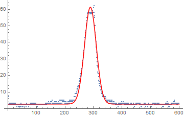
Data and normal curve regression fit

$\endgroup$
10
  • $\begingroup$ It is worth noting that you added a parameter in the fit (the constant value a0). This reduces the error but it is no longer a pure Gaussian. $\endgroup$
    – anderstood
    Commented Oct 27, 2017 at 16:02
  • $\begingroup$ @anderstood I did state "What you can do is add another parameter that raises the curve a bit to get a more appropriate regression fit." but you're right, I should make that more explicit. But why fit a "pure Gaussian" when it clearly isn't? I'm waiting for a response from the OP to find out if this is a regression problem or a fitting of a probability distribution from a random sample. Those are two very different beasts. $\endgroup$
    – JimB
    Commented Oct 27, 2017 at 16:06
  • $\begingroup$ I agree that your model is much more relevant in most cases :). I just thought it might be out of scope (not sure). $\endgroup$
    – anderstood
    Commented Oct 27, 2017 at 16:17
  • $\begingroup$ @anderstood. What part of my answer is “out of scope”? $\endgroup$
    – JimB
    Commented Oct 27, 2017 at 17:06
  • 2
    $\begingroup$ @anderstood. Got it. However, I feel (but maybe I shouldn’t) that answering what the question ought to be is fair game. I do try to restrict that urge to just statistical abuses. And mixing regression and estimation of probability distributions is a common abuse. $\endgroup$
    – JimB
    Commented Oct 27, 2017 at 17:59

Your Answer

By clicking “Post Your Answer”, you agree to our terms of service and acknowledge you have read our privacy policy.

Not the answer you're looking for? Browse other questions tagged or ask your own question.