Curved mesh boundary from space curve

Question

This is a follow-up question to an earlier question.

Question: Given a general space curve xy[t_] = {x[t], y[t]}, how can a region be generated to yield a mesh with a curved boundary? (A related question has appeared before, but is more specialized.)

Background: An implicitly defined boundary (i.e. an exact curve) allows a better representation of a region, as compared to one generated the usual way (from a set of points connected by line segments). This fact is demonstrated by comparing the area of exact and numerical regions. See Documentation (“Region Approximation Quality”).

Consider, for simplicity, a circular boundary:

Needs["NDSolve`FEM`"]    
R = ImplicitRegion[x^2 + y^2 <= 1, {x, y}];
nr = ToNumericalRegion[R];
mesh1 = ToElementMesh[nr];
AreaExact = Pi;
AreaExact - Total[mesh1["MeshElementMeasure"], 2]

2.00118*10^-6

Now compare this to building a custom mesh. A crude approach is to extract a sequence of points, and use them as boundary nodes (let us take this number equal to the number of nodes of mesh1).

Nt = Length[DeleteDuplicates[Flatten[mesh1["BoundaryElements"][[1, 1]]]]];
xy[t_] = {Cos[t], Sin[t]};
coords = Table[N[xy[(2 Pi)/Nt i]], {i, 0, Nt - 1}];
LElms = Table[{Mod[i + 2, Nt, 1], i, i + 1}, {i, 1, Nt - 1, 2}]; 
bm = ToBoundaryMesh["Coordinates" -> coords, 
  "BoundaryElements" -> {LineElement[LElms]}]; 
mesh2 = ToElementMesh[bm];
AreaExact - Total[mesh2["MeshElementMeasure"], 2]

0.00896404

Because the region R is defined implicitly, i.e. using ImplicitRegion, information about the curvature of the boundary is automatically passed during the call to ToElementMesh, and mesh1 is endowed with a curved boundary, making it a better approximation of the region. For the custom mesh (mesh2), a piecewise linear boundary (polygonal) results, causing a large “error” in the area.

Note that the error scales quadratically with 1/Nt, whereas, for comparison, the implicit region error scales as the fourth order of "MaxBoundaryCellMeasure” parameter.

Assuming a xy[t] is smooth, one would guess that simply interpolating the points during the construction of the mesh boundary would be a significant improvement to the "polygonal" approximation since the order of interpolation could match the order of the mesh itself. Can this be done? If not, is there a reason why? (I understand that one sometimes requires non-differentiable points, e.g. corners, on the boundary, but surely such points can be accommodated.)

Note that I have explored using ParametricRegion:

xy[ρ_, t_] = ρ xy[t];
R = ParametricRegion[xy[ρ, t], {{t, 0, 2 Pi}, {ρ, 0, 1}}];

However, this seems to require a full coordinate mapping xy[ρ,t] depending on a "radial" coordinate ρ, i.e. it is not addressing the stated problem. Furthermore, the error seems no better than the polygonal approximation:

nr3 = ToNumericalRegion[R];
mesh3 = ToElementMesh[nr3];
AreaExact - Total[mesh3["MeshElementMeasure"], 2]

0.0033998

Answer 1

After some reflection, I believe I have a solution to the above question. I'm happy with the result, although, to be fair, it is a rather massive hack. Perhaps (hopefully!) the functionality will simply be added to Mathematica at some point...

Restatement of problem: For the purpose of making a mesh, the "precise" boundary curvature of a region can be encoded into a numerical region. Unfortunately, this information seems to be too deep "under the hood" of Mathematica, so cannot be added manually. As far as I can tell, the only tool available to us to pass information about boundary curve is via the use of ImplicitRegion. Thus, we must accept this constraint, and the original question can be restated --

Q: Given a general closed curve in 2D, xy[t] (periodic in the variable t), how does one generate the corresponding enclosed region using ImplicitRegion.

The problem seems to be that it is hard to translate a space curve xy[t] into simple Boolean-valued function in terms of x and y that is needed for input to ImplicitRegion. My idea was to break the boundary up, so that such a function could be defined in a piecewise fashion.

For illustrative purposes, we will consider a circular boundary (note that this can easily be turned into a single Boolean function using polar coordinates, but there are many perfectly nice space curves that cannot):

Needs["NDSolve`FEM`"]
xy[t_] = {Cos[t], Sin[t]};
xyP[t_] = D[xy[t], t];

Some simple but useful functions:

ci[i_, Nt_] := Mod[i, Nt, 1]
Contains[x_, Domain_] := Domain[[1]] <= x <= Domain[[2]]

We must identify a number of points on the boundary for the purpose of constructing a "scaffolding" (see the figure later). This number doesn't need to be that big -- it need only be large enough that the boundary does not "curve too much" and a single-valued function can locally be built to implicitly define the boundary curve.

Nt = 10;
Rf = 2;(* Resampling factor *)
Stf = 1/2;(* Scafolding thickness factor *)

We now make a list of boundary points and tangent unit vectors at those points. A second, more dense set of t-points is chosen for sampling the boundary curve; the accuracy of the final mesh will depend on the density of the second set (set by Rf), not the first.

tList = Table[N[i/Nt 2 Pi], {i, 0, Nt - 1}];
tList2 = Table[N[i/(Rf Nt) 2 Pi], {i, 0, Rf Nt - 1}];
Bcoords = Table[N[xy[ti]], {ti, tList}];
tanVecs = Table[N[xyP[ti]]/Norm[xyP[ti]], {ti, tList}];

We will project along the normal direction at each boundary node, both inward and outward, to create an inner and outer polygonal regions. From this, a set of quadrilateral cells will be defined. (As long as the values of tList are sufficiently dense, and the boundary curve smooth, the boundary curve will be contained between the inner and outer polygons.)

coordsOuter = {}; coordsInner = {};
For[i = 1, i <= Nt, i++,
  l = Stf (Norm[Bcoords[[ci[i, Nt]]] - Bcoords[[ci[i - 1, Nt]]]] + 
      Norm[Bcoords[[ci[i + 1, Nt]]] - Bcoords[[ci[i, Nt]]]])/2; 
  (* choose size of scaffolding using distance to neighboring points *)
  tv = tanVecs[[i]];
  n = {tv[[2]], -tv[[1]]};(* n = t x Overscript[z, ^] *)
  AppendTo[coordsOuter, Bcoords[[i]] + l n];
  AppendTo[coordsInner, Bcoords[[i]] - l n];
];

Now we construct a set of "condition functions", one for each cell, that can be used to build a global function to be given as input to ImplicitRegion. These functions are not boolean-valued but are smooth because ImplicitRegion prefers this.

The functions will not be expressed exactly in terms of xy[t], but instead using Interpolation with a number of points (determined by resampling factor Rf). (This seems fine, since the ultimate application is to building a mesh which can only be second order itself.)

ConditionFcns = {};
For[i = 1, i <= Nt, i++,
  (* Make a scaffolding cell *)
  (* points of bounding polygon listed counterclockwise from top right *)
  boundingPts = {coordsOuter[[ci[i, Nt]]], 
    coordsOuter[[ci[i + 1, Nt]]], coordsInner[[ci[i + 1, Nt]]], 
    coordsInner[[ci[i, Nt]]]};
  (* Set up local Cartesian coords for building Y[X] fcn *)
  b = Bcoords[[i]]; a = Bcoords[[ci[i + 1, Nt]]];
  c = (a + b)/2;(* coord center *)
  Xhat = (b - a)/Norm[b - a]; 
  Yhat = {-Xhat[[2]], Xhat[[1]]};
  tl = Table[tList2[[ci[j, Rf Nt]]], {j, Rf (i + 1), Rf ( i - 1), -1}];
  Ydata = Table[{(xy[t] - c).Xhat, (xy[t] - c).Yhat}, {t, tl}];
  YI = Interpolation[Ydata]; Dom = YI["Domain"][[1]];
  AppendTo[ConditionFcns, 
   If[Contains[Xhat.({x, y} - c), Dom], 
    Evaluate[-Yhat.({x, y} - c) + YI[Xhat.({x, y} - c)]], -1]];
];

Now we will have to stitch together all these functions into a single global function. To do this we will need a method of locating first which (if any) cell a given $x$-$y$ point is contained in. Let's use the inPoly function suggested by @R.M.

inPolyQ[poly_, pt_] := Graphics`PolygonUtils`PointWindingNumber[poly, pt] =!= 0

Define inner and outer polygonal regions:

cInnerPadded = Append[coordsInner, First[coordsInner]]; 
cOuterPadded = Append[coordsOuter, First[coordsOuter]];
PInner = Polygon[coordsInner];
POuter = Polygon[coordsOuter];

We construct a function getIndex that returns the index of the cell containing point {x,y}. It returns $i \in 1\dots N_t$ if the point is contained in a boundary cell i. It returns $0$ if the point is contained in PInner. Otherwise it gives $-1$. It is basically a binary search algorithm.

getIndex[x_, y_] := 
 If[inPolyQ[PInner, {x, y}], 0, 
  If[inPolyQ[POuter, {x, y}], WhichCell[x, y, 1, Nt], -1]]
getPoly[iMin_, iMax_] := 
 Polygon[Join[Take[cOuterPadded, {iMin, iMax + 1}], 
   Reverse[Take[cInnerPadded, {iMin, iMax + 1}]]]]
WhichCell[x_, y_, iMin_, iMax_] := Module[{i2 = Floor[(iMin + iMax)/2]},
  If[inPolyQ[getPoly[iMin, i2], {x, y}],
   If[iMin == i2, iMin, WhichCell[x, y, iMin, i2]],
   If[i2 + 1 == iMax, iMax, WhichCell[x, y, i2 + 1, iMax]]]
  ]
For[i = 1, i <= Nt, i++, cLFcn[x_, y_, i] = ConditionFcns[[i]];]

Define the global function to give to ImplicitRegion.

inΩN[x_?NumericQ, y_?NumericQ] := Module[{i = getIndex[x, y]},
  Which[i == -1, -1, i == 0, 1, i > 0, cLFcn[x, y, i]]
  ]

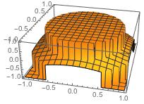
Can verify visually that it is smooth within the boundary cells.

Plot3D[inΩN[x, y], {x, -1, 1}, {y, -1, 1}, 
 PlotPoints -> 100]

Finally we get to build the mesh!

rbs = RegionBounds[POuter];
RS = ImplicitRegion[inΩN[x, y] >= 
   0, {{x, rbs[[1, 1]], rbs[[1, 2]]}, {y, rbs[[2, 1]], rbs[[2, 2]]}}];
nrS = ToNumericalRegion[RS];
meshS = ToElementMesh[nrS];

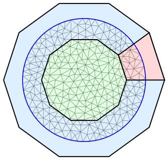
Let's visualize the whole process as follows. We show the inner polygon (green) and outer polygon (blue) together with a one of the quadrilateral boundary cells (pink), the boundary curve (blue) and the corresponding region constructed with ImplicitRegion (mesh):

Show[
 Graphics[{{EdgeForm[Thick], LightBlue, POuter}, {EdgeForm[Thick], 
    LightGreen, PInner}, {EdgeForm[Thick], LightRed, getPoly[1, 1]}}],
  ParametricPlot[xy[t], {t, 0, 2 Pi}, Axes -> False, 
  PlotStyle -> Blue], 
 meshS["Wireframe"["MeshElementStyle" -> EdgeForm[Thin]]]]

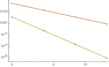
Finally, we would like to demonstrate that this whole process was worth the effort. Let us show how well the new mesh gives the area of the unit circle. We calculate the error in the usual way as

AreaError[m_] := Pi - Total[m["MeshElementMeasure"], 2]

Fixing Nt = 10, we vary Rf. A polygonal mesh is built for comparison

meshP = ToElementMesh[
   Polygon[Table[N[{Cos[ti], Sin[ti]}], {ti, tList2}]]];

So the accuracy is not to be limited by the size of the boundary mesh cells, we use a refined boundary mesh in what follows:

meshS = ToElementMesh[nrS, "MaxBoundaryCellMeasure" -> 0.05];

A log-log plot demonstrates the error scales as $R_f^{-4}$ for the new mesh, as compared to $R_f^{-2}$ for the polygonal approximation:

SError

{{2, 0.00330491}, {4, 0.000206049}, {8, 0.0000128467}, {16, 7.98742*10^-7}}

PError

{{2, 0.0514227}, {4, 0.0129034}, {8, 0.00322882}, {16, 0.000807393}}

FitP = Table[{PError[[i, 1]], 
    PError[[1, 2]] (PError[[i, 1]]/PError[[1, 1]])^-2}, {i, 1, 
    Length[PError]}];
FitS = Table[{SError[[i, 1]], 
    SError[[1, 2]] (SError[[i, 1]]/SError[[1, 1]])^-4}, {i, 1, 
    Length[SError]}];
ListLogLogPlot[{SError, FitS, PError, FitP}, 
 Joined -> {False, True, False, True}]

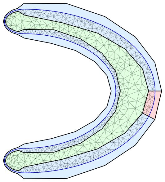
EDIT: Here a nontrivial space curve to demonstrate the method works generally.

xyE[θ_, el_] := {el Cos[θ], Sin[θ]};
xy[t_, wf_, el_] := Module[{θ},
   Which[
    0 <= t < Pi/2, θ = 2 t - Pi/2; xyE[θ, el],
    Pi/2 <= t < Pi, θ = 
     2 t - Pi/2; (1 - wf)/2 xyE[θ, el] + {0, (1 + wf)/2},
    Pi <= t < 3 Pi/2, θ = 5 Pi/2 - 2 t; wf xyE[θ, el],
    3 Pi/2 <= t <= 2 Pi, θ = 
     2 t - 5 Pi/2; (1 - wf)/2 xyE[θ, el] - {0, (1 + wf)/2}
    ]
   ];
xyEP[θ_, el_] := {-el Sin[θ], Cos[θ]};
xyP[t_, wf_, el_] := Module[{θ},
   Which[
    0 <= t < Pi/2, θ = 2 t - Pi/2; 2 xyEP[θ, el],
    Pi/2 <= t < Pi, θ = 2 t - Pi/2; 
    2 (1 - wf)/2 xyEP[θ, el],
    Pi <= t < 3 Pi/2, θ = 
     5 Pi/2 - 2 t; -2 wf xyEP[θ, el],
    3 Pi/2 <= t <= 2 Pi, θ = 2 t - 5 Pi/2; 
    2 (1 - wf)/2 xyEP[θ, el]
    ]
   ];
wf = 0.7; el = 1.6;
xy[t_] := xy[t, wf, el];
xyP[t_] := xyP[t, wf, el];

Set global parameters

Nt = 40;
Rf = 3;(* Resampling factor *)
Stf =  1/4;(* Scafolding thickness factor *)

Visualize the result like before:

ii = 5; Show[
 Graphics[{{EdgeForm[Thick], LightBlue, POuter}, {EdgeForm[Thick], 
    LightGreen, PInner}, {EdgeForm[Thick], LightRed, 
    getPoly[ii, ii]}}], 
 ParametricPlot[xy[t], {t, 0, 2 Pi}, Axes -> False, 
  PlotStyle -> Blue], 
 meshS["Wireframe"["MeshElementStyle" -> EdgeForm[Thin]]]]