Uniform distribution on z = 1 − √( x ^2 + y ^2) , z ≥ 0 [duplicate]

Question

Let $S$ belong to ${\rm I\!R^3}$, $z = 1 − \sqrt{x^2 + y^2}$ , $z ≥ 0$.

I need to write a program that generates a random point on $S$ with uniform distribution. I've tried to use

g[z_, fi_] = {(1 - z)*Cos[2 Pi*fi], (1 - z)*Sin[2 Pi*fi], z};
sample[n_] := Table[g[RandomReal[], RandomReal[]], {n}];

sampleX[n_] := Table[g[RandomReal[], RandomReal[]][[1]], {n}];
sampleY[n_] := Table[g[RandomReal[], RandomReal[]][[2]], {n}];
sampleZ[n_] := Table[g[RandomReal[], RandomReal[]][[3]], {n}];  

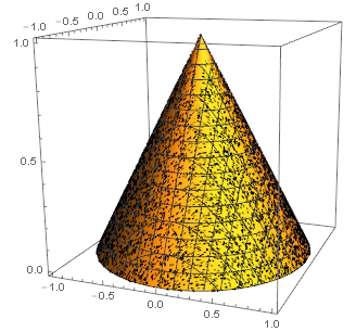
But the result isn't exact, because I have more points on the top and less points near $OXY$.

How could I make a Uniform distribution on this surface?

Answer 1

If you set up your region S as a region in Mathematica you can use RandomPoint to generate uniformly distributed points over it.

reg = ImplicitRegion[
   z == 1 - Sqrt[(x^2 + y^2)], {{x, -1, 1}, {y, -1, 1}, {z, 0, 1}}];
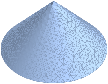
dreg = DiscretizeRegion[reg]
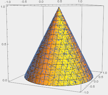
rp = RandomPoint[dreg, 10000];
Show[ContourPlot3D[
  z == 1 - Sqrt[(x^2 + y^2)], {x, -1, 1}, {y, -1, 1}, {z, 0, 1}], 
  Graphics3D[{PointSize[0.05], Point[rp]}]]

This should be fine for most purposes, but note that the discretised region dreg is a numerical approximation to the ImplicitRegion, reg. So, for example

point = RandomPoint[dreg]
RegionMember[dreg, point]
RegionMember[reg, point]

(* {-0.538245, -0.716972, 0.103292}
   True
   False *)

That is, while point in the discretised region, dreg, it is not actually in the implicit region reg. Although it is close:

RegionDistance[reg, point]

(* 0.000129349 *)

The approximation of the mesh in dreg could be improved with MaxCellMeasure.

In case you're wondering, sadly we can't just generate RandomPoints from reg:

RandomPoint[reg]

(* RandomPoint[ImplicitRegion[z == 1 - Sqrt[x^2 + y^2] && -1 <= x <= 1 && -1 <= y <= 1 && 0 <= z <= 1, {x, y, z}]] *)

It "should" work (according to documentation), but Region functionality in Mathematica often has funny quirks to it.

UPDATE: Comparison of approaches to uniform distributions over a region embedded in a higher dimensional space

There have been two general approaches to generating uniformly distributed random points over the surface of a cone. @Coolwater and @george2079 opted for analytical solutions, while @Carl Woll and myself used Mathematica's built in Region functionality. I wanted to have a look at how these approaches compare in accuracy and speed; and get a sense of how best to approach similar problems.

An important feature of this question is that the region dimension is less than the embedding dimension (and this is the reason for the woeful accuracy of RandomPoint applied to DiscretizeRegion; if RegionDimension == EmbeddingDimension accuracy shouldn't be a problem). With this in mind, the take-home message based on the table below seems to be:

1. Keep to analytical solutions as far as possible. A little math goes a long way.
2. If you must use Regions, use the ParametricRegion or built-in ones.
3. Use ImplicitRegion and DiscretizeRegion only in emergencies.

First, a few definitions:

carlreg = 
  RegionIntersection[RegionBoundary[Cone[{{0, 0, -1}, {0, 0, 1}}, 2]],
    ConicHullRegion[{0, 0, 0}, {{1, 0, 0}, {0, 1, 0}}, {{0, 0, 1}}]];
implicitreg = 
  ImplicitRegion[
    z == 1 - Sqrt[x^2 + y^2], {{x, -1, 1}, {y, -1, 1}, {z, 0, 1}}];
discreg = DiscretizeRegion[implicitreg];
parareg = 
  ParametricRegion[{Cos[θ] u, Sin[θ] u, 1 - u}, 
    {{θ, 0, 2 π}, {u, 0, 1}}];

coolwater[n_] := 
 Transpose[{Cos[#] #2, Sin[#] #2, 1 - #2} &[RandomReal[2 π, n], 
   Sqrt[RandomReal[1, n]]]]
george[n_] := 
 Append[#1 Through[{Sin, Cos}@#2], 1 - #1] & @@@ 
  Transpose[{RandomVariate[ProbabilityDistribution[2 r, {r, 0, 1}], 
     n], RandomReal[{0, 2 π}, n]}]
carlwoll[n_] := RandomPoint[carlreg, n]
aardvark[n_] := RandomPoint[discreg, n]
parametric[n_] := RandomPoint[parareg, n]

Now generate some points

{names, timing, points} = 
  Transpose[Join[{#}, AbsoluteTiming[#[1000]]] & /@ 
    {coolwater, george, carlwoll, aardvark, parametric}];
regdist = Mean[RegionDistance[implicitreg, #]] & /@ points;
solerror = Mean[Abs[#3 - (1 - Sqrt[#1^2 + #2^2])] & @@@ #] & /@ points;
TextGrid[Join[{{"", "Timing", "RegionDistance", "Solution error"}}, 
  Transpose[{names, timing, regdist, solerror}]]]

\begin{array}{|c|ccc|} \hline \text{} & \text{Timing} & \text{RegionDistance} & \text{Solution error} \\ \hline \text{coolwater} & 0.0003290 & 1.25468 \times 10^{-10} & 1.68754 \times 10^{-17} \\ \text{george} & 0.0049363 & 1.66830 \times 10^{-10} & 1.87628 \times 10^{-17} \\ \hline \text{carlwoll} & 0.0458737 & 5.67581 \times 10^{-10} & 6.13953 \times 10^{-17} \\ \text{aardvark} & 0.0006388 & 0.000600271 & 0.000849862 \\ \text{parametric} & 0.0251807 & 7.21428 \times 10^{-11} & 1.74305 \times 10^{-17} \\ \hline \end{array}

A few words about the difference between implicitreg, parareg and @CarlWoll's carlreg. They are clearly the same mathematical region, their Region-based properties (RegionMeasure, RegionCentroid, etc) are identical, and FindInstance cannot find any points that they do not all have in common. However, RandomPoint can be used directly on carlreg and parareg but not on implicitreg. I don't have an explanation why that is the case, but it is possibly related to this question by @rhermans. Basically, ImplicitRegions are much more complicated for Mathematica to work with. So using them for a case like this, where there are many other options, is clearly (in hindsight) a mistake.

Answer 2

The radius increase linearly w.r.t. t = 1-z, so the cumulative distribution function is t^2. Hence transforming uniform variables for t by the square root (the quantile) makes the result uniform.

samp[n_] := Transpose[{Cos[#] #2, Sin[#] #2, 1 - #2} &[
              RandomReal[2 π, n], Sqrt[RandomReal[1, n]]]]

surf = ContourPlot3D[z == 1 - Sqrt[x^2 + y^2], {x, -1, 1}, {y, -1, 1}, {z, 0, 1}];
Show[surf, ListPointPlot3D[samp[9000]]]

Answer 3

Your surface is just the boundary of a cone (excluding the base), and RandomPoint will work with the region boundary of a Cone object. We can intersect the region boundary of a slightly extended cone with a region with $z>0$ to eliminate the base. RandomPoint will also work with this region intersection object. So, I will use a cone with a circle of radius 2 at $(0, 0, -1)$ as the base and $(0, 0, 1)$ as the top, so that the intersection with $z>0$ is the desired cone:

reg = RegionIntersection[
    RegionBoundary[Cone[{{0, 0, -1}, {0, 0, 1}}, 2]],
    ConicHullRegion[{0, 0, 0}, {{1, 0, 0}, {0, 1, 0}}, {{0, 0, 1}}]
];

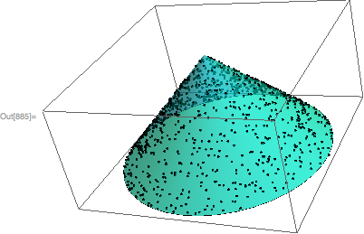
pts = RandomPoint[reg, 1000];

Graphics3D[{Point@pts, RGBColor[0, 1, 1, .5], Cone[{{0, 0, 0}, {0, 0, 1}}]}]

And, here is a check that pts satisfy the desired equation:

Tally @ Chop[Function[{x, y, z}, z - (1 - Sqrt[x^2+y^2])] @@@ pts]

{{0, 1000}}

Answer 4

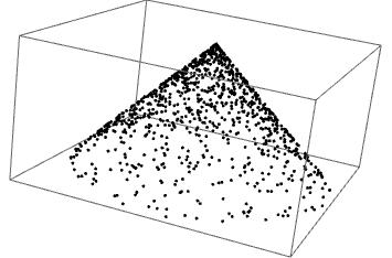
small tweak using RandomVariate :

n = 10^3
ListPointPlot3D[
 Append[#1 Through[{Sin,Cos}@#2], 1 - #1] & @@@ 
 Transpose[{
   RandomVariate[ProbabilityDistribution[2 r , {r, 0, 1}], n],
   RandomReal[{0, 2 Pi}, n]}]]