Plotting a complicated vector field

Question

If we consider the vector $\left ( A \cdot \nabla \right) \: B$, we have in Cartesian coordinates

$$\left ( A \cdot \nabla \right) \: B = \left ( A \cdot \nabla B_x \right ) e_x + \left ( A \cdot \nabla B_y \right ) e_y + \left ( A \cdot \nabla B_z \right ) e_z,$$ which gives in full writing:

$$\left ( A \cdot \nabla \right) \: B = \left (A_x \frac{\partial \: B_x}{\partial \: x} + A_y \frac{\partial \: B_x}{\partial \: y} + A_z \frac{\partial \: B_x}{\partial \: z} \right )e_x + \left (A_x \frac{\partial \: B_y}{\partial \: x} + A_y \frac{\partial \: B_y}{\partial \: y} + A_z \frac{\partial \: B_y}{\partial \: z} \right )e_y + \left (A_x \frac{\partial \: B_z}{\partial \: x} + A_y \frac{\partial \: B_z}{\partial \: y} + A_z \frac{\partial \: B_z}{\partial \: z} \right )e_z$$

Now, say $B=A$ and $A=\left (10 \: x, \: 20 \, y^3, \: 30 \:z \right )$.

I would like to plot the field of $A$ and of $\left ( A \cdot \nabla \right) \: A$ in Mathematica. How to go about?

(My objective in this exercise is to know which direction the vector $\left ( A \cdot \nabla \right) \: A$ lies with respect to $A$ and also test for different vectors $A$ when the lines of $\left ( A \cdot \nabla \right) \: A$ are straight or are curved.)

Thanks a lot...

Answer 1

Update since version 9 Grad is built in.

Let us first define the vector field

A = {10 x, 20 y^3, 30 z};

and load the vector analysis package:

Now let's define $A\cdot \nabla A$

field = (A.Grad[#, {x, y, z}]) & /@ A

(* ==> {100 x, 1200 y^5, 900 z} *)

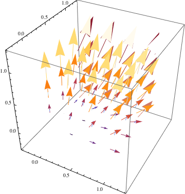
and plot both fields:

pl1 = 
  VectorPlot3D[A, {x, 0, 1}, {y, 0, 1}, {z, 0, 1}, 
   VectorColorFunction -> "Heat", VectorPoints -> Coarse];

pl2 = 
  VectorPlot3D[field, {x, 0, 1}, {y, 0, 1}, {z, 0, 1}, 
   VectorColorFunction -> "ThermometerColors", VectorPoints -> Coarse];

Show[pl1, pl2]

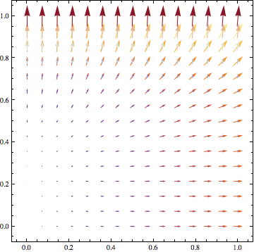
We could also look at a slice

{VectorPlot[Most[A], {x, 0, 1}, {y, 0, 1}, 
   VectorColorFunction -> "Heat"],
  VectorPlot[Most[field], {x, 0, 1}, {y, 0, 1}, 
   VectorColorFunction -> "ThermometerColors"]} // Show

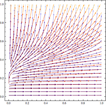
Or using a different plotting function, StreamPlot:

pl1 = StreamPlot[Most[A], {x, 0, 1}, {y, 0, 1}, 
   StreamColorFunction -> "SolarColors"];
pl2 = StreamPlot[Most[field], {x, 0, 1}, {y, 0, 1}, 
   StreamColorFunction -> "LakeColors"];

Show[pl1, pl2]

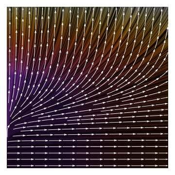
Or yet another, LineIntegralConvolutionPlot (takes a bit longer)

pl1 = LineIntegralConvolutionPlot[{Most[A], {"noise", 800, 800}}, {x, 
    0, 1}, {y, 0, 1}, ColorFunction -> "Heat", LightingAngle -> 0, 
   LineIntegralConvolutionScale -> 3, Frame -> False];

pl2 = StreamPlot[Most[field], {x, 0, 1}, {y, 0, 1}, 
   StreamColorFunction -> Function[x, White]];

Show[pl1, pl2]