Orientation of the pattern in an image

Question

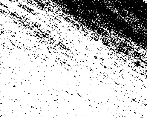
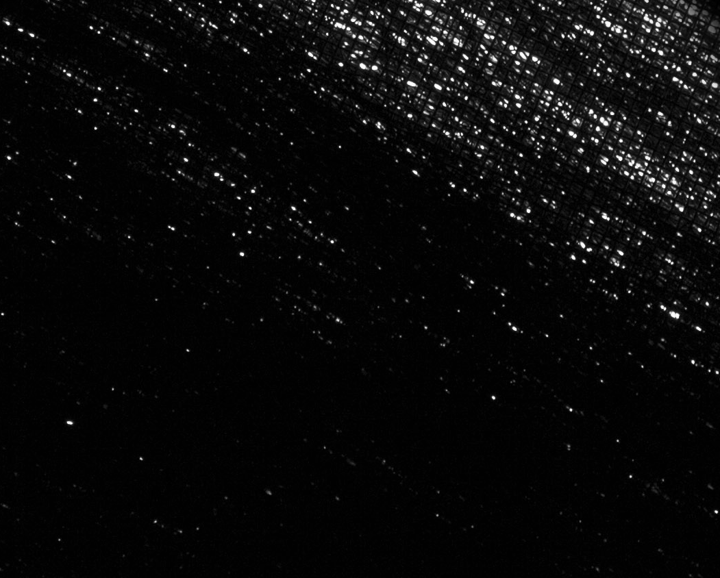
Following the topic Find the center of a circular specimen, I have trouble determining the principal orientations of the pattern in an image: Image to analyze

The main goal was to find the principal direction of the pattern in an image and to orient the image accordingly. So far, I have tried to use the code from Mathematica Image Processing tutorial (Analyze Orientations in an Image) and an SE answer bellow the following link: Image Processing: Finding Orientation and Position of Symmetry Axes

However, both methods are not working as they should and images have to be rotated manually with ImageRotate. In this example image would have to be rotated for approximately 45° in order to align the pattern principal orientation axes with the horizontal and vertical directions.

I think that the main problem is small size of white pockets without dominant dimension. Global orientation of the pattern can only be seen when looked upon an image from far away.

EDIT

It is important to add that I am looking for the orientation of white-spot pattern and not the orientation of the rectangular net. Nevertheless, your suggestions are really nice, because they deal with problem from different angles.

Before reading your answers I was trying to do something considering the comments from @nikie. What I found out was that the EdgeDetect is very sensitive to the r parameter definition. Besides, "RANSAC" method in ImageLines turned out to be a better predictor than the default "Hough" method.

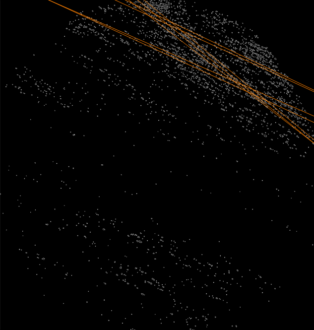
With the code: Show[EdgeDetect[Binarize@imageC, 2], Graphics[{Orange, Line /@ ImageLines[EdgeDetect[Binarize@imageC, 2], Method -> "RANSAC"]}], ImageSize -> Large] following results were obtained:

And with the code: Show[Binarize@imageC, Graphics[{Orange, Line /@ ImageLines[Binarize@imageC, Method -> "RANSAC"]}], ImageSize -> Large] following lines were obtained:

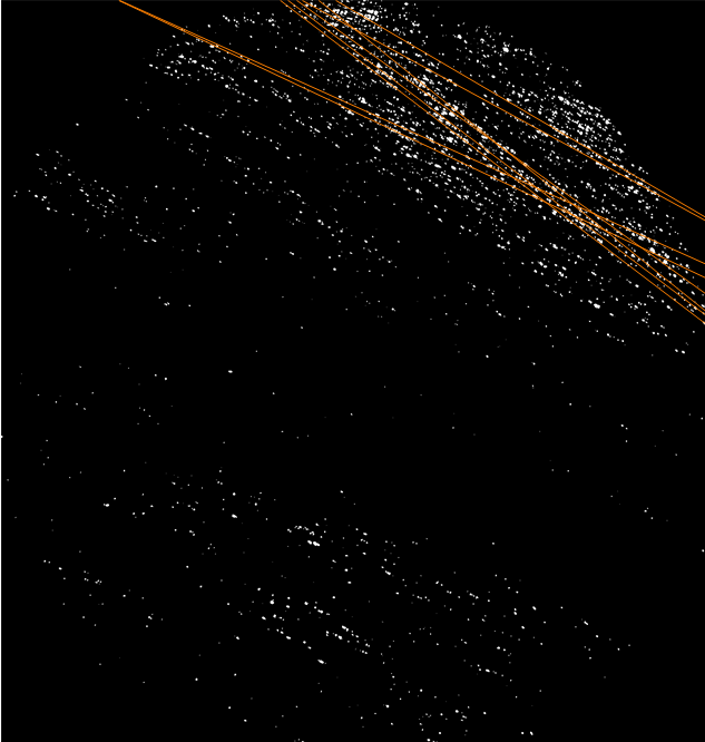
As already mentioned, the change of method to "RANSAC" with default t and d parameters was crucial improvement in the quality of the results. In this case we have a lot of outliers in the data and "RANSAC" is more suitable in assigning no influence to them than the "Hough" method. I will try your suggestions, too, in order to get the best method for line-pattern recognition.

Answer 1

I see two possible solutions here. You can either use the orientation of the white spots to calculate the mean orientation of them all. The other possibility is to acknowledge that there is an underlying grid which is probably what you call pockets.

Let's first try to enhance them

img = Import["https://i.sstatic.net/KAJ7r.png"];
Manipulate[
 Binarize[img, {t1, t2}],
 {t1, 0, 1},
 {t2, t1, 1}
 ]

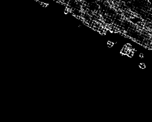
Beside the large portion of white in the bottom part, the grid becomes visible. Let us use this image and kill the white portion

Manipulate[
 ImageMultiply[Binarize[img, {0, t}], 
  Binarize[GaussianFilter[img, g]]],
 {{t, 0.04}, 0, 0.1},
 {{g, 20}, 3, 30}
 ]

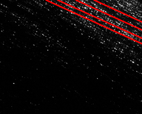
That looks like a good start for ImageLines

lines = ImageLines[
   ImageMultiply[Binarize[img, {0, 0.04}], 
    Binarize[GaussianFilter[img, 30]]]];
HighlightImage[img, {Red, Thickness[0.01], Line /@ lines}]

Answer 2

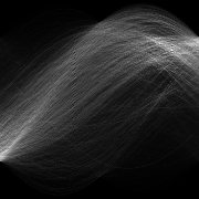
One approach is using the Radon transform:

img = Import["https://i.sstatic.net/KAJ7r.png"];
rad = Radon[img, {180, 180}];
ImageAdjust[rad]

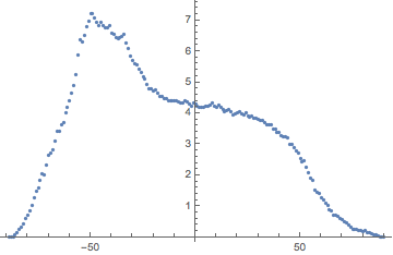
The column of the Radon matrix with the largest sum is the direction with the strongest line:

xaxis = Range[-89, 90];
radDat = ImageData[rad];
trans = Total[Transpose[radDat]];
ListPlot[Transpose[{xaxis, trans}]]
pos = First@First@Position[trans, Max[trans]];
xaxis[[pos]]

-50

which shows that the strongest sum is at about -50 degrees, the amount to rotate the image so that the stripes are vertical.

Answer 3

You can use the code from this question more or less without changes:

img = Import["https://i.sstatic.net/KAJ7r.png"];

pixels = ImageData[img];

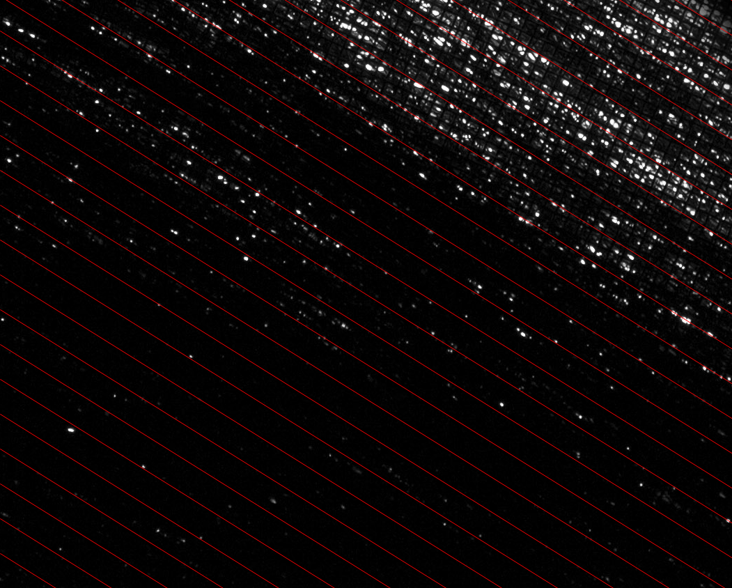
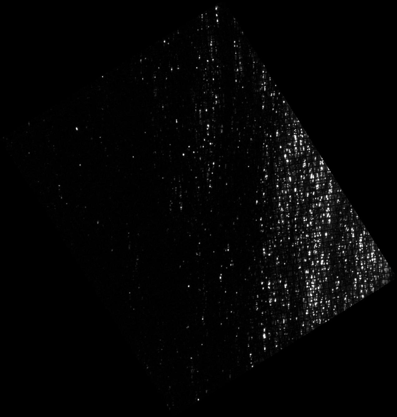
The idea is basically: Treat the gradient (strength and direction) as complex numbers, square them, so gradient vectors pointing in opposite directions have the same phase, then sum them up:

sigma = 10; (*roughly the with of a line*)
gradient = 
  GaussianFilter[pixels, sigma, {0, 1}] + 
   I GaussianFilter[pixels, sigma, {1, 0}];

sumSquaredGradient = Total[gradient^2, \[Infinity]];

angle = Arg[Sqrt[sumSquaredGradient]]

{w, h} = ImageDimensions[img];
Show[ImageAdjust[img], 
 Graphics[{Red, 
   Table[Line[{{0, y}, {w, w*Cot[angle] + y}}], {y, 0, 2 h, 50}]}]]

ImageRotate[img, angle]

Answer 4

Since we have GradientOrientationFilter,the thing become easer.

img = Import["https://i.sstatic.net/KAJ7r.png"];
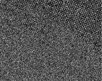
orient = GradientOrientationFilter[img, 3]

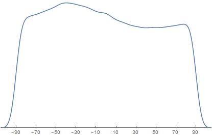
angles = Rescale[Flatten[ImageData[orient]], {-Pi/2, Pi/2}, {-90, 90}];
SmoothHistogram[angles, Axes -> {True, False}, 
 Ticks -> {Range[-90, 90, 20]}]