Update: Found a simpler way to get a first approximation to minimax polynomial.
On MiniMaxApproximation[] and the OP's f[h]
The file
FileNameJoin[{$InstallationDirectory, "AddOns", "Packages",
  "FunctionApproximations", "Approximations.m"}]
contains several hundred lines of documentation, discussion and examples. You may wish to consult it for alternatives to what I shall present.
The file warns that functions with singular points can be difficult, if not impossible. I'm not sure if infinite singularities are what they have in mind, or any sort of discontinuities in the function or its first two derivatives (which are used in the algorithm!). The suggestion is to modify the function so that it is more amenable to the algorithm. The example they give is subtracting out a logarithmic singularity, approximating the difference, and adding the singularity back in.
The order-2 interpolation has a discontinuous second derivative:
Plot[{f[h], 10000 f'[h], 10000^2 f''[h]}, {h, 0, 50000},
 PlotLabel -> Row[{"Interpolation Order ", f["InterpolationOrder"]}]]

One can bump up the interpolation order to 3 or 4 and get smooth derivatives, but MiniMaxApproximation[] still fails. So I suspected the problem might be arising from a combination of a few issues:
- the oscillation around 14000-16000 (most apparent in
f''[h]) or perhaps other less obvious oscillations from the interpolation.
- the exponential decrease in the value of
f[h] over the interval (over a factor 1000), which makes minimizing the relative error more difficult.
- the potential rounding error over such a long interval (
h^5 can be as big as 3.125*^23).
Since Exp[-c h] can be approximated (for c small enough to avoid underflow but large enough that the value changes by a factor of 1000 or more), it cannot simply be the last two. It seems more likely that the little oscillation introduces extra extrema once the degree of the polynomial is sufficiently high and the polynomial is somewhat close to f[h]. MiniMaxApproximation[] cannot figure out which extrema should be ignored and the function fails. In the OP's case, there is one too many extrema (by the Equioscillation Theorem), which is a pickle because no matter which one is dropped -- and it cannot be one of the end points -- the signs will not alternate. This should have suggested that the starting point was bad, but at first, I did not know you could set the starting point of MiniMaxApproximation[].
mmaOP = MiniMaxApproximation[f[h], {h, {0, hMax}, 5, 0}];

Plot[(f[h] - mmaOP[[2]])/(1 + 0 f[h]), {h, 0, 50000},
 GridLines -> {mmaOP[[1]], None},
 PlotLabel -> "Error of failed minimax"]

The file also suggests that in difficult cases, it may be possible to approach the minimax polynomial by a sequence of approximations, such as by approximating f[h] to get good starting values for MiniMaxApproximation[] or by starting with a smaller interval and extending it.
Obtaining the minimax approximant
To get the minimax approximant, I started with an exponential model, since the data looks like a decaying exponential, by forming the interpolation logf of the logarithm of the data rdata. The Chebyshev series approximant mma0 to the interpolation logf was found à la Boyd/Chebfun (see this answer). I then used the MiniMaxApproximation[] to mma0 as the starting point for finding the minimax approximant to f[h].
logf = Interpolation[
   MapAt[Log, rdata, {All, 2}],      (* take the Log of the function values *)
   InterpolationOrder -> 2, Method -> "Spline"];

Block[{n = 8},  (* Chebyshev interpolation on 2n+1 points *)
  cnodes = Rescale[Sin[Pi/2 N@Range[-n, n]/n], {1, -1}, {0, hMax}];
  yy = logf@cnodes;
  cc = Sqrt[1/n] FourierDCT[yy, 1];
  cc[[{1, -1}]] /= 2;
  mma0 = Exp[cc[[;; 6]].ChebyshevT[Range[0, 5], 2 h/hMax - 1]]
  ] // Simplify
(*
  1.20576 E^(h (-0.0000759961 - 4.3012*10^-9 h + 9.65032*10^-14 h^2 -
      9.43409*10^-19 h^3 + 4.03776*10^-24 h^4))
*)

era = MiniMaxApproximation[mma0, {h, {0, 50000}, 5, 0}];     (* initial approximation *)
mma = MiniMaxApproximation[f[h], era, {h, {0, hMax}, 5, 0}]  (* fed as second argument *)
mma = %[[2, 1]];                                             (* extract the approximant *)
(*
  {{0., 10288.8, 18883.7, 31749.7, 41032.1, 47359., 50000.},
   {1.27756 - 0.000135637 h + 5.86599*10^-9 h^2 - 1.28016*10^-13 h^3 +
     1.40093*10^-18 h^4 - 6.12305*10^-24 h^5,
    -0.0429097}}
*)

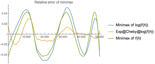
Plot[{(f[h] - era[[2, 1]])/f[h], (f[h] - mma0)/f[h], (f[h] - mma)/f[h]},
 {h, 0, 50000},
 PlotStyle -> {Automatic, Automatic, Thick},
 PlotLabel -> "Relative error of minimax",
 PlotLegends -> {Row[{"Minimax of ", HoldForm@Log[f[h]]}],
   Row[{"Exp@Cheby@", HoldForm@Log[f[h]]}],
   Row[{"Minimax of ", HoldForm@f[h]}]}]

Note the exponential/Chebyshev/logarithmic approximant is better than the minimax. Of course, you would need an Exp[] function in your actual application to use it. One can also see how the wobbliness of the interpolation is magnified and might create extra extrema; a higher interpolation order produces a somewhat smoother error plot.


