To draw several histogram in a temporal axis

Question

I have 1000 histograms obtained from a Monte-Carlo complex simulation process. So to explain what I am searching I will simplify my problem.

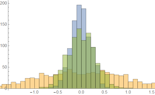
If I want to draw 3 histograms on the same scale, I will write a program like the following one

h1 = RandomVariate[NormalDistribution[], 1000];
h2 = RandomVariate[NormalDistribution[0, .2], 1000];
h3 = RandomVariate[NormalDistribution[0, .3], 1000];
Histogram[{h1, h2, h3}]

which will gives

But, this graphic is not easy to read and there is a third temporal axis, since all distributions are obtained step after step. So I would add a third axis and draw the histogram obliquely with the 0 of the two others axes situated on the third one, as is the usage for stochastic processes.

Thanks for the help

Answer 1

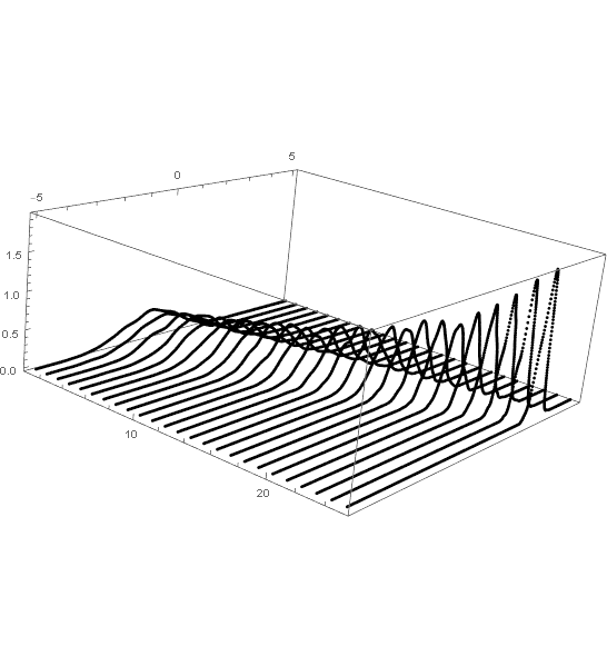
To emphasize my comment: when one wants to display many histograms, one really needs to use nonparametric density estimators. Here's an example:

nSimulations = 25;
nSamples = 1000;  (* Sample size for each pdf *)
n = 1000;  (* Number of points for drawing each pdf *)
pdfs = ConstantArray[0, {nSimulations, n}];
μ = Table[-1. + 4 (i - 1)/(nSimulations - 1), {i, nSimulations}];
σ = Table[1. - 0.8 (i - 1)/(nSimulations - 1), {i, nSimulations}];
Do[h = SmoothKernelDistribution[RandomVariate[NormalDistribution[μ[[i]], σ[[i]]], nSamples]];
 pdfs[[i]] = Table[{i, x, PDF[h, x]}, {x, -5, 5, 10/n}],
 {i, nSimulations}]

ListPointPlot3D[pdfs, PlotRange -> All, PlotStyle -> Black]

Answer 2

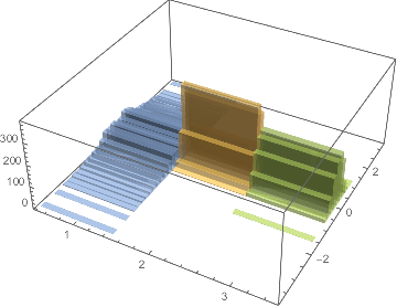
One approach is to use Histogram3D:

Histogram3D[{Transpose@{ConstantArray[1, Length[h1]], h1}, 
  Transpose@{ConstantArray[2, Length[h2]], h2}, 
  Transpose@{ConstantArray[3, Length[h3]], h3}}]

More generally, if you place all your data in a big matrix:

h = {h1, h2, h3}; 
Histogram3D[Transpose[{ConstantArray[#, Length[h[[#]]]], h[[#]]}] & /@ Range[3]]

then you can plot all 1000 data sets just by changing the parameter in the Range function.