Why is my parallel version of `DensityPlot` slow?

Question

I am exploiting the possibility to parallelize DensityPlot.

This is my naive implementation

Clear[parallelDensityPlotData];
parallelDensityPlotData[func_, xrange_, yrange_, partition_, 
  opts : OptionsPattern[]] := Module[{x, y},
  extractPlot3Ddata[graphics_] := graphics[[1, 1]];
  newXrangeList = 
   Partition[Subdivide[Sequence @@ xrange, partition[[1]]], 2, 1];
  newYrangeList = 
   Partition[Subdivide[Sequence @@ yrange, partition[[2]]], 2, 1];
  newRangeList = Tuples[{newXrangeList, newYrangeList}];
  rangeToParaRange = Flatten /@ {{x, #[[1]]}, {y, #[[2]]}} &;
  paraRangeList = rangeToParaRange /@ newRangeList;
  graphicsList = 
   ParallelTable[
    Plot3D[func[x, y], Evaluate[Sequence @@ i], Mesh -> None, 
     PlotRange -> All, 
     Evaluate@FilterRules[{opts}, Options[Plot3D]]], {i, 
     paraRangeList}];
  ListDensityPlot[
   Partition[Flatten[extractPlot3Ddata /@ graphicsList], 3], 
   Evaluate@FilterRules[{opts}, Options[ListDensityPlot]]]]

It is a simple implementation that partition the whole rectangle into smaller rectangle and Plot3D on each rectangle, then extract the each data, do a final ListDensityPlot.

However, I found my implementation just can't compete with serial running DensityPlot.

For example, take function from this post

f[x_, y_] := (x^2 + y^2) Exp[-x^2 - y^2] Sin[10 Sqrt[x^2 + y^2] + 10 ArcTan[x, y]]^4;

then

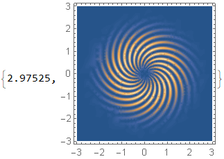
DensityPlot[f[x, y], {x, -3, 3}, {y, -3, 3}, PlotPoints -> 24, 
  PlotRange -> All, MaxRecursion -> 3] // AbsoluteTiming

While

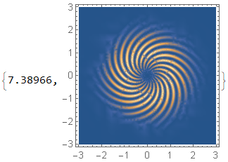
parallelDensityPlotData[f, {-3, 3}, {-3, 3}, {3, 3}, PlotPoints -> 8, 
  MaxRecursion -> 3, PlotRange -> All] // AbsoluteTiming

Though, I only have two cores, but this is kind of slow.

My guess is that Plot3D takes too much time calculating other things?

So I am wondering what is the core adaptive part function inside Plot3D so that we can directly use? I've tried to use PrintDefinitions, but got lost in the output.