25
$\begingroup$

Cross posted to Wolfram Community


Mathematica has a layout algorithm to plot planar graphs without edge crossings. This typically produces an ugly triangular layout where some vertices and edges are nearly overlapping (even if technically they do not intersect).

@JasonB posted this example in chat:

g = Graph[EdgeList@ChemicalData["FullereneC60", "StructureGraph"], 
  GraphLayout -> "PlanarEmbedding"]
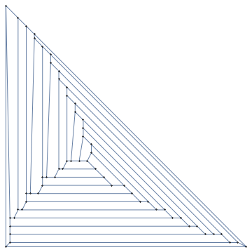
Mathematica graphics

How can we create a more pleasing visualizaton of planar graphs than this?

GraphData has the same fullerene graph with much nicer vertex coordinates included:

GraphData[{"Fullerene", {60, 1}}]
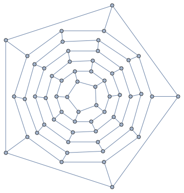
Mathematica graphics

How could we create something comparable (if not quite as symmetric) automatically?

I am looking for practical methods. They do not need to work on all planar graphs, and it is okay if they need manual tuning. But they should be practically useful for visualizing some large class of planar graphs.


GraphData["Planar"] gives a long list of graphs that you can use for testing. GraphData["Planar", 20] gives some planar graphs with 20 vertices.

Some graphs will plot well (and without edge crossings) using a simple SpringElectricalEmbedding, even when the method in the below answer fails on them. An example is GraphData[{"SierpinskiCarpet", 4}].

One particularly challenging graph is GraphData[{"Apollonian", 5}]. Can you plot this one nicely?


Bounty update:

There may be multiple different approaches which work in specific situations only. Feel free to post these as well. One possibility is using a SpringElectrical type embedding in 3D, then projecting it down to the plane in such a way as to maintain symmetries (which is the hard part: projecting is easy, maintaining symmetries is not).

Since more than one method may work, and since methods that only work on a subclass of graphs may have high practical utility, I may award additional smaller bounties to good answers even after the 300 bounty is gone.

$\endgroup$
10
  • 1
    $\begingroup$ I would suggest simulated annealing on the vertex coordinates, with an aim to reduce the combined length of the edges (perhaps just the sum, perhaps a more nuanced measure) as small as possible -- while of course avoiding crossings. I'm underwater with other work, no time to poke around and cobble it together, but maybe that's a start. $\endgroup$ Commented Apr 26, 2017 at 21:53
  • $\begingroup$ @KellenMyers Something like this? $\endgroup$
    – Szabolcs
    Commented Apr 26, 2017 at 22:28
  • 1
    $\begingroup$ @Rahul I was hoping to see other ideas, or pure Mathematica implementations. That solution does not work that well, and requires a lot of manual fussing. $\endgroup$
    – Szabolcs
    Commented Apr 27, 2017 at 8:10
  • 4
    $\begingroup$ "TutteEmbedding" can help... $\endgroup$
    – halmir
    Commented Apr 27, 2017 at 13:32
  • 1
    $\begingroup$ By the way I don't think the fullerene in GraphData is the same as $C_{60}$. The central pentagon is adjacent to five other pentagons. $\endgroup$
    – user484
    Commented Apr 27, 2017 at 18:30

2 Answers 2

17
$\begingroup$

One possibility is to first lay out the graph using Mathematica's "PlanarEmbedding". This ensures no edge crossings, but the output is not pleasing. Then use the Davidson–Harel algorithm through IGraph/M to refine the result.

The Davidson–Harel algorithm uses simulated annealing to try to optimize the layout, and includes a penalty for edge crossings. On its own, it would not be able to disentangle the edges and eliminate all crossings. However, this implementation allows using existing coordinates as starting vertex positions through the "Continue" option (most IGraph/M layout algorithms have this). We use the coordinates from "PlanarEmbedding" and increase the penalty for edge crossings. It does not always work, but it tends to perform reasonably on not too large graphs.

Demonstration

We start by selecting all planar graphs that have at least 15 vertices and are not trees or forests (i.e. they are acyclic). Trees are too easy to layout, thus boring.

gs = GraphData /@ GraphData["Planar"];    
gs = Select[gs, VertexCount[#] > 15 && Not@AcyclicGraphQ[#] &];

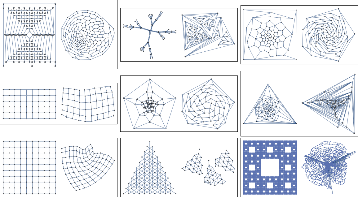
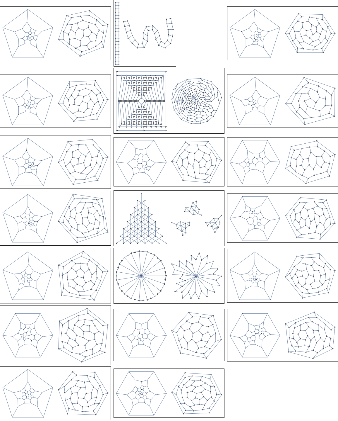
Let us try the method on 20 random ones. In each box, the left figure shows the original layout in GraphData. This layout is often hand-made, and can be taken as a reference point for what sort of nice visualization is possible for the given graph. The right side shows the layout automatically computed by this method.

<<IGraphM`

SeedRandom[52];
IGSeedRandom[52]; 
Table[Framed@Grid@List@{
   Graph[g, ImageSize -> Small], 
   IGLayoutDavidsonHarel[
       SetProperty[g, 
         VertexCoordinates -> 
         Thread[VertexList[g] -> 
           Rescale@
            GraphEmbedding[g, 
             "PlanarEmbedding"]]],
       "Continue" -> True, "EdgeCrossingWeight" -> 1000, 
       ImageSize -> Small]}, {g, RandomSample[gs, 20]}] // 
 Multicolumn[#, 3] &

enter image description here

Unfortunately, on larger graphs, it won't work quite as well, even after tuning the parameters. There is clearly plenty of room for improvement, so I am still looking for alternative answers, including simulated annealing implementations in pure Mathematica.

gs = GraphData /@ GraphData["Planar"];
gs = Select[gs, VertexCount[#] > 59 && Not@AcyclicGraphQ[#] &];

SeedRandom[52];
IGSeedRandom[52]; 
Table[Framed@
   Grid@List@{Graph[g, ImageSize -> Small], 
      IGLayoutDavidsonHarel[
       SetProperty[g, 
        VertexCoordinates -> 
         Thread[VertexList[g] -> 
           2 Rescale@
             GraphEmbedding[g, 
              "PlanarEmbedding"]]],(*unpack to work around bug*)
       "Continue" -> True, "EdgeCrossingWeight" -> 50000, 
       MaxIterations -> 100, ImageSize -> Small]}, {g, 
   RandomSample[gs, 9]}] // Multicolumn[#, 3] &

enter image description here

$\endgroup$
2
  • 1
    $\begingroup$ Well,do mean the latter is a pleasing way? :) $\endgroup$
    – yode
    Commented Apr 27, 2017 at 10:11
  • $\begingroup$ @yode The coordinates in the left picture come from GraphData. In the right hand side picture they are automatically computed. $\endgroup$
    – Szabolcs
    Commented Apr 27, 2017 at 10:49
5
+150
$\begingroup$

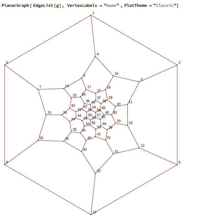
There is a Built-in function PlanarGraph introduced in 2016 (10.4) that does the job. It automatically creates something comparable to the output of GraphData[{"Fullerene", {60, 1}}]. It is also possible to write a function that uses simple pattern matching to change the distance and position of nodes. This link to an article's section about planar graph embedding puzzles offers a useful reference; it features a small interactive interface that could be refactored to solve precisely that.

g = Graph[EdgeList@ChemicalData["FullereneC60", "StructureGraph"], 
  GraphLayout -> "PlanarEmbedding"];

enter image description here
PlanarGraph should work to visualize a relatively large class of planar graphs, however, internally it only seems to be choosing between GraphLayout -> "TutteEmbedding" and GraphLayout -> "PlanarEmbedding" based on whether KVertexConnectedGraphQ[g, 3] is True. Using the particularly challenging graph as an example to take a closer look:
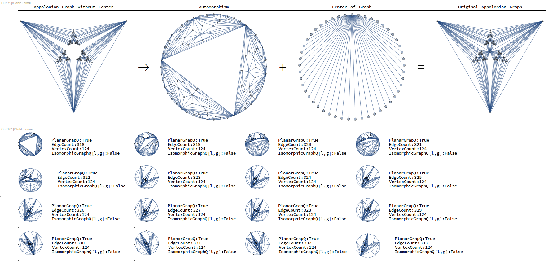
PlanarGraph[EdgeList@GraphData[{"Apollonian", 5}], PlotTheme -> "Classic"]
even after some manual tuning the resulting planar graph is in a similar initial situation:

planar = PlanarGraph[ EdgeList@GraphData[{"Apollonian", 5}]];
  v1 = GraphEmbedding[planar];
  v2 = VertexCoordinates /. AbsoluteOptions[planar, VertexCoordinates];
  v3 = PropertyValue[{g, #}, VertexCoordinates] & /@ VertexList[g];
  v4 = Cases[Show[planar], DiskBox[x_, y__] :> x, {0, Infinity}];
  vcplanar = GraphEmbedding[planar, "PlanarEmbedding"];
  SetProperty[planar, VertexCoordinates -> vcplanar];
  SetProperty[planar, GraphLayout -> "PlanarEmbedding"]


Removing certain vertices and edges just to add them manually later using some other method seems to improve the GraphLayout 's option default behavior when using PlanarGraph but still does not solve the initial problem. The Handbook of Graph Drawing and Visualization is a good reference to implement a graph drawing algorithm; it aims at providing a broad survey of the field of graph drawing. It covers topological and geometric foundations, algorithms, software systems, and visualization applications for business, education, science, and engineering.

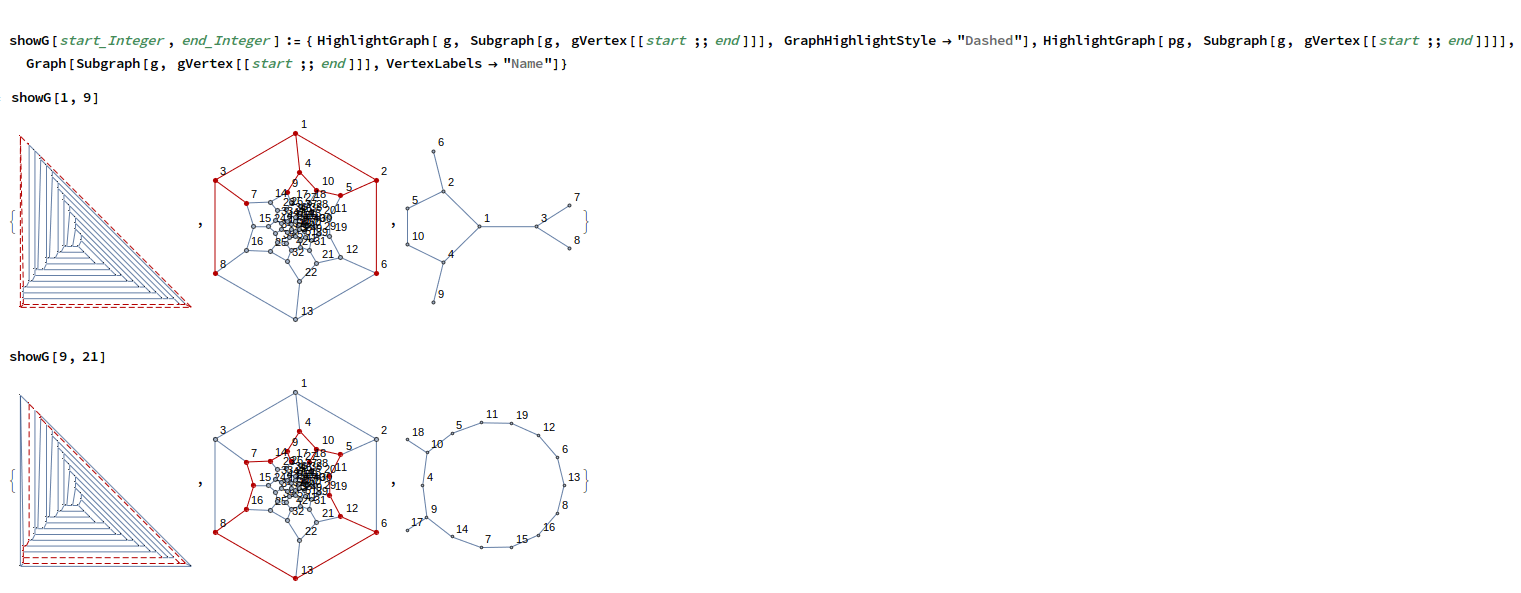
We can verify results in steps by comparing subgraphs or at once simply using IsomorphicGraphQ.

g = Graph[EdgeList@ChemicalData["FullereneC60", "StructureGraph"], 
  GraphLayout -> "PlanarEmbedding"]; pg = 
 PlanarGraph[EdgeList@ChemicalData["FullereneC60", "StructureGraph"], 
  VertexLabels -> "Name"]; 
showG[start_Integer, end_Integer] := { 
  HighlightGraph[ g, Subgraph[g, EdgeList[g][[start ;; end]]], 
   GraphHighlightStyle -> "Dashed", VertexLabels -> "Name"], 
  HighlightGraph[ pg, Subgraph[g, EdgeList[pg][[start ;; end]]]], 
  Graph[Subgraph[g, EdgeList[g][[start ;; end]]], 
   VertexLabels -> "Name"]}

enter image description here

$\endgroup$
1
  • 4
    $\begingroup$ Isn't PlanarGraph simply choosing between GraphLayout -> "TutteEmbedding" and GraphLayout -> "PlanarEmbedding" based on whether KVertexConnectedGraphQ[g, 3]? In this case it just uses the Tutte embedding. $\endgroup$
    – Szabolcs
    Commented May 9, 2017 at 7:14

Your Answer

By clicking “Post Your Answer”, you agree to our terms of service and acknowledge you have read our privacy policy.

Not the answer you're looking for? Browse other questions tagged or ask your own question.