Small positive eigenvalues found for a negative definite matrix

Question

I have encountered a problem with Mathematica that I really don't know how to solve. I'm sorry if I am going to be very verbose but I need it to explain the problem properly (and also make the code I'm going to show more comprehensible).

I'm using Mathematica to work for my master's thesis and in these days I'm dealing with the ecosystem model described in this article. Amongst the things I have to do there's the study of the eigenvalue distribution of the community matrix of this ecosystem, i.e. the jacobian matrix of the system of coupled ODEs that describe the population abundances of the various species, computed at the steady state of the system.

In a single sentence my problem is the following: as the size of this matrix increases Mathematica finds that it has also very small positive eigenvalues, while this matrix is always definite negative.

More in detail (now I have to be very verbose): the model describes a system of $m$ animal species competing for $p$ resources. These resources are supplied with constant rates $\vec{s}=(s_1,\dots,s_p)$, and every species can be identified with its metabolic strategy $\vec{\alpha}_{\sigma}=(\alpha_{\sigma 1}, \dots, \alpha_{\sigma p})$ (where $\sigma=\{1,\dots,m\}$ labels the species, and $\alpha_{\sigma i}$ can be interpreted as the ratio at which species $\sigma$ eats resource $i$). Now, assuming $m \geq p$ and that $\vec{\alpha}_\sigma$-s (properly renormalized) satisfy $$\sum_{i=1}^p \alpha_{\sigma i} = 1 \quad \forall \sigma$$ (called "metabolic trade-off condition") it can be shown that the system is stable (i.e. all species survive) if $\vec{s}$ belongs to the convex hull of metabolic strategies, i.e. if: $$\exists \{n_1^*>0, \dots, n_m^*>0\} : \sum_{\sigma=1}^m n_\sigma^* = 1 \quad \text{and} \quad \vec{s} = \sum_{\sigma=1}^m n_\sigma^* \vec{\alpha}_\sigma$$ Now, studying the model analytically it turns out that the jacobian matrix of the system computed at this stable steady state can be written as: $$\mathcal{M}=-DASA^T$$ where: $$D=\operatorname{diag}(n_1^*, \dots, n_m^*) \qquad S=\operatorname{diag}(1/s_1,\dots,1/s_p) \qquad A_{\sigma i} = \alpha_{\sigma i}$$ and it can be shown that for $m \geq p$ it is always definite negative.

Now, with Mathematica I'm trying to study numerically the eigenvalue distribution of $\mathcal{M}$. The code I am using in order to do so is the following:

m = 1000;
p = m;
A = #/Total[#, {2}] &@RandomReal[{0, 1}, {m, p}];       
\[ScriptCapitalN] = (#/Total[#, {2}] &@RandomReal[{0, 1}, {1, m}])[[1]];
S = Sum[\[ScriptCapitalN][[i]]*A[[i]], {i, 1, m}];
\[ScriptCapitalD] = DiagonalMatrix[\[ScriptCapitalN]];
\[ScriptCapitalS] = DiagonalMatrix[1/S];
\[ScriptCapitalM] = -\[ScriptCapitalD].A.\[ScriptCapitalS].Transpose[A];
eigenvalues = Eigenvalues[\[ScriptCapitalM]];
ListPlot[{Re[#], Im[#]} &/@ eigenvalues, PlotRange -> Automatic]
Length[Select[eigenvalues, # > 0 &]]
Max[eigenvalues]

(I added the last two lines to keep track how many eigenvalues are positive and which is the largest eigenvalue).

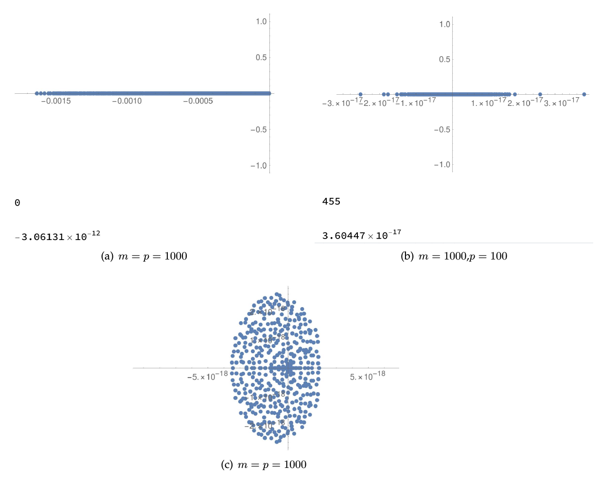
Now, If I set $m=p$ no problems arise and all eigenvalues are indeed negative. For example, for $m=p=1000$ I get the plot in figure $a)$ (below).

However, problems start popping up if I set $m > p$ (which is the most interesting case for the model). In fact, the results of the analytical study of $\mathcal{M}$ (i.e. the fact that it's negative definite) are valid for $m \geq p$, but using the code I have written it happens that some eigenvalues start "collapsing" around 0, and they turn out to be both positive and negative (even if very very small in magnitude). The number of "collapsed" eigenvalues increases as the ratio $m/p$ increases, until they become the majority of the eigenvalues.

For example, if I use the same code with $m=1000$ and $p=100$ I get figure $b)$ below.

My question is therefore the following: is there something am I doing wrong in the code? Or is this just a problem of numerical precision?

I first thought it could be the latter, so I have tried to increase the numerical precision a bit by changing the third and fourth line of the previous code to:

 A = #/Total[#, {2}] &@
   RandomReal[{0, 1}, {m, p}, WorkingPrecision -> 7];
\[ScriptCapitalN] = (#/Total[#, {2}] &@
     RandomReal[{0, 1}, {1, m}, WorkingPrecision -> 7])[[1]];

However, new problems arise: apart from the fact that computation now requires a lot more time (I had to use much smaller values of $m$ and $p$ in order to get results in minutes) the eigenvalues are now complex, instead of purely real! For example, for $m=500$; $p=80$ I get figure $c)$ below.

Therefore, if this is indeed a problem of numerical precision, how can I fix it? Is there a more efficient way to increase it?

Here are the plots:

Sorry again for the verboseness.

Answer 1

Your first matrix is negative definite. Your second one has rank 100 and dim 1000x1000, so it is negative semidefinite. The smallest in magnitude eigenvalue for the first is around 10^(-11), so it is sufficiently distinct from machine arithmetic fuzz that it is not messed up by numeric error. The 900 zero eigenvalues in the second one are not going to be found as exact zeros by any numerical method, and that's why there is a fairly symmetric range of machine fuzz values appearing around the origin.