How to generate approximately equally spaced points efficiently

Question

I don't very content with current method.So a better solution is expected still.I hope it meet two conditions in following.

1. That space is approximately equivalence.
2. We can control how many points to produce.

---

v11.1 provides a new function SpherePoints. As the Details

SpherePoints[n] gives exactly equally spaced points in certain cases for small n. In other cases, it places points so they are approximately equally spaced.

Can we achieve the same goal i.e. approximately equally spaced points in an arbitrary 2D Region?

The following is my attempt based on Union:

SeedRandom[1]
region = ConvexHullMesh[RandomReal[1, {100, 2}]];
UniformPts = 
  Union[RandomPoint[region, 50000], 
   SameTest -> (EuclideanDistance[#1, #2] < .1 &)];
Show[region, Graphics[Point[UniformPts]]]

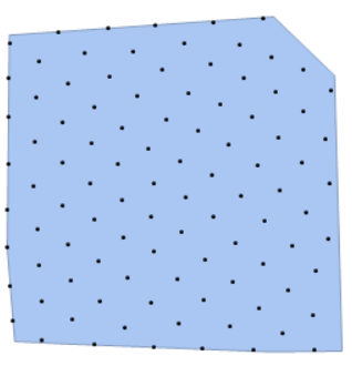
Nevertheless, this approach has two weakness:

1. It is slow with a large number of pre-generated points i.e. the 2nd argument of RandomPoint, while the space won't be uniform enough if I don't pre-generate enough points, here's an example:

   

2. The number of resulting points isn't controllable.

Answer 1

Annealing

Found this to be an interesting question and immediately I thought it to be a good application for simulated annealing.

Here's a little unoptimized annealing function I wrote. The idea is that your points move around like atoms in random directions but they "cool down" over time and move less and settle into a minimum energy configuration state.

My rules are:

1. plan a move in a random direction and random distance of maximum length step
2. move only if the distance to the nearest point increases
3. move only if the new location is inside the region

Assumes rm is a globally defined RegionMember function.

anneal[pts_, step_] := 
 Module[{np, nn, test1, test2, pl, potentialMoves},
  pl = Length@pts;
  np = Nearest@pts;
  nn = np[#, 2][[2]] & /@ pts;
  potentialMoves = RandomReal[step, pl]*RandomPoint[Circle[], pl];
  test1 = 
   Boole@Thread[
     MapThread[EuclideanDistance[#1, #2] &, {pts, nn}] < 
      MapThread[
       EuclideanDistance[#1, #2] &, {pts + potentialMoves, nn}]];
  test2 = Boole[rm /@ (pts + potentialMoves)];
  pts + potentialMoves*test1*test2]

Here is an example with 200 pts, 1000 steps and an anneal rate of .995. Initial step should be on the order of the region size:

Clear[x,y];reg=ImplicitRegion[x^2-y^2<=1,{{x,-3,3},{y,-3,3}}];
rm=RegionMember[reg];
pts=RandomPoint[reg,200];
step=1;
Do[pts=anneal[pts,step=.995*step],1000];
Show[RegionPlot[reg],Graphics[{Black,Point/@pts}]]

Here is an animation of the process:

Answer 2

Many solutions similar to how to get $n$ equidistributed points on the unit sphere are possible, especially if one can accept that points are not on the edges of a region. For instance, one can use analytical Lloyd's method:

With[{reg = RegularPolygon[5]}, 
 Nest[RegionNearest[reg][
     RegionCentroid@RegionIntersection[reg, #] & /@ 
      MeshPrimitives[VoronoiMesh@#, 2]] &, RandomPoint[reg, 20], 20] //
   Graphics[{LightBlue, reg, Black, Point@#}] &]

This is awfully slow, though.

A much faster variant is to use a Monte Carlo method to estimate Voronoi cell centroids:

With[{reg = RegularPolygon[5]}, 
 With[{points = 500, samples = 40000, iterations = 20}, 
   Nest[With[{randoms = Join[#, RandomPoint[reg, samples]]}, 
      RegionNearest[reg][
       Mean@randoms[[#]] & /@ 
        Values@PositionIndex@Nearest[#, randoms]]] &, 
    RandomPoint[reg, points], iterations]] // 
  Graphics[{LightBlue, reg, Black, Point@#}] &]

A more complex concave example (which benefits from higher iteration count) as suggested by @J.M.:

With[{reg = 
   Cases[Graphics`PolygonUtils`PolygonData[
      "HexaSpiral"], _Polygon, \[Infinity]][[1]]}, 
 With[{points = 500, samples = 40000, iterations = 200}, 
   Nest[With[{randoms = Join[#, RandomPoint[reg, samples]]}, 
      RegionNearest[reg][
       Mean@randoms[[#]] & /@ 
        Values@PositionIndex@Nearest[#, randoms]]] &, 
    RandomPoint[reg, points], iterations]] // 
  Graphics[{LightBlue, reg, Black, Point@#}] &]

Answer 3

This does not give you real control over the number of points, but its one way to get somewhat equally spaced distribution of points:

region = ConvexHullMesh[RandomReal[1, {100, 2}]];
<< NDSolve`FEM`
elementMesh = ToElementMesh[region, MeshQualityGoal -> 0];
coordinates = elementMesh[[1]];
triangles = elementMesh[[2, 1, 1]];
centers = 
  Table[
    Sum[{coordinates[[triangles[[i, j]], 1]],coordinates[[triangles[[i, j]], 2]]}, {j, 1, 3}]/3
   , {i, 1, Length[triangles]}];
Show[region, Graphics[Point[centers]]]

Update

Trivial solution, but seems to be relatively quick:

numberOfPoints = 500;
region = BoundaryDiscretizeGraphics[Text["K"], _Text];
<< NDSolve`FEM`
elementMesh = ToElementMesh[region, MeshQualityGoal -> 0];
coordinates = Transpose[elementMesh[[1]]];
Xmin = Min[coordinates[[1]]];
Xmax = Max[coordinates[[1]]];
Ymin = Min[coordinates[[2]]];
Ymax = Max[coordinates[[2]]];
scale = (Xmax - Xmin + Ymax - Ymin)/2;
spacing = scale/40;
test[x_] := RegionMember[region, x];
points := DeleteCases[
  Flatten[Table[ If[test[{i, j}], {i, j}, -1], {i, Xmin, Xmax, spacing}, {j, Ymin, Ymax, spacing}], 1] 
  , -1];
(
 data = Table[{1/(spacing = ii scale/300), points // Length} // Reverse, {ii, 10, 20}];
 fun[x_] = NonlinearModelFit[data, a + b x^(1/2), {a, b}, x] // Normal;
 spacing = 1/fun[numberOfPoints];
 (pts = points) // Length
) // AbsoluteTiming
Show[region, Graphics[Point[pts]]]

{0.187837, 505}

We can see that within 0.188 seconds we have generated a distribution of 505 points where we tried to generate a 500 points distribution. The error in number of points is always just a few percent at the most.

Answer 4

Since Mma v12.2 spatial point processes have opened yet another possibility with HardcorePointProcess, which prevents processes from resulting points being pairwise closer than a specified distance from each other. This is not to such an extent a "packing" as many other answers to this question, since only minimum distance is constrained, but it does demonstrate that there are multiple ways to approach the question. Consider, for instance:

With[{reg = 
   Cases[
     Graphics`PolygonUtils`PolygonData[
      "HexaSpiral"], _Polygon, \[Infinity]][[1]]}, 
 Graphics[{LightBlue, reg, Black,
   Point@RandomPointConfiguration[
      HardcorePointProcess[10000, 2, 2],
      reg, Method -> {"LengthOfRun" -> 10000000}]["Points"]}]]

Here the number of points produced is somewhat random, but depends on the region area, the specified point density (the first argument to HardcorePointProcess) and the minimum distance constraint (the second argument).

Answer 5

Rebuilt and little refine for this answer

equPoint[region_, pointNum_] := 
 Module[{pts, stepDist, rm, regionRange, beFar, InRegion, moveDir}, 
  pts = RandomPoint[region, pointNum];
  rm = RegionMember[region];
  regionRange = 
   EuclideanDistance @@ Transpose[RegionBounds[region]]/100;
  stepDist = Subdivide[regionRange, 0, 500];
  moveDir = 
   RandomReal[#, pointNum]*RandomPoint[Circle[], pointNum] & /@ 
    stepDist;
  Fold[(beFar = 
      Boole@Thread[
        EuclideanDistance @@@ Nearest[#, #, 2] < 
         EuclideanDistance @@@ Nearest[#1 + #2, #1 + #2, 2]];
     InRegion = Boole[rm /@ (#1 + #2)];
     # + #2*beFar*InRegion) &, N[pts], moveDir]]

Explanation

I have not iterated 1000 times,but make the difference of the last two times less the pre,whose default value is 0.001,after 500 times.And you don't need to consider the size of region.

Example

region = ImplicitRegion[x^2 - y^2 <= 1, {{x, -3, 3}, {y, -3, 3}}];
BoundaryDiscretizeRegion[region, 
 Epilog -> {Point[equPoint[region, 200]]}]

Here is an animation of the process: