72
$\begingroup$

Mathematica produces fantastic-looking graphics, but it can be slow on large data sets. Here is an example for a (random) time series:

rv = RandomVariate[ExponentialDistribution[2], 10^5];

Plotting this takes quite some time:

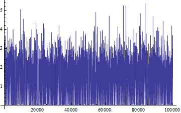
t = AbsoluteTime[]; ListLinePlot[rv, PlotRange -> All]
AbsoluteTime[] - t (* Put this line into the NEXT cell, and evaluate both cells together*)

Mathematica graphics

The option PerformanceGoal->"Speed" has no effect. Turning off antialiasing makes it much faster (but if you increase the data size to 10^6 instead of 10^5, it is still VERY slow. A time series of 10^6 points is quite reasonable in my applications):

t = AbsoluteTime[]; 
Style[ListLinePlot[rv, PlotRange -> All], Antialiasing -> False]
AbsoluteTime[] - t (* This line in separate cell! *)

Mathematica graphics

Reducing the number of MaxPlotPoints makes it much faster, but completely distorts the shape of the data:

t = AbsoluteTime[]; ListLinePlot[rv, PlotRange -> All, MaxPlotPoints -> 1000]
AbsoluteTime[] - t (* This line in separate cell! *)

Mathematica graphics

Question: I am interested in tricks to show the data quickly without distorting the shape. I am showing here my own solution, which is quite a bit of a hack, but it works. Are there more elegant solutions?

Edit:

My own answer, previously posted as part of the question, is now an independent answer (see below)

$\endgroup$
6
  • 3
    $\begingroup$ FYI you can use Timing or AbsoluteTiming to time the execution of a command, instead of having to subtract time values manually. $\endgroup$
    – David Z
    Commented Jan 18, 2012 at 11:19
  • 1
    $\begingroup$ I don't think it works for the plotting, as Timing[] only reports about the time spent in the Kernel. $\endgroup$
    – Thomas
    Commented Jan 18, 2012 at 12:08
  • $\begingroup$ Oh, maybe I misunderstood your question. Are you asking about the time it takes the resulting Graphics object to render on screen? AbsoluteTiming might cover that as well, since it measures wall time, not CPU time, though I forget when exactly it stops. (BTW, if rendering is the bottleneck, saving the plot to a rasterized image file can be a good strategy) $\endgroup$
    – David Z
    Commented Jan 18, 2012 at 12:17
  • 7
    $\begingroup$ @David AbsoluteTiming[] doesn't cover rendering of the graphic. It only times how long it takes for the kernel to finish, and the rendering is done by the front end only after the Graphics expression has been sent to it. Generally, both Timing and AbsoluteTiming measure the time it takes for the kernel to finish (not front end), but the former is CPU time while the latter is wall time. $\endgroup$
    – Szabolcs
    Commented Jan 18, 2012 at 12:23
  • $\begingroup$ @NasserM.Abbasi To be honest, I am not completely clear about these either. I do know that AbsoluteTiming won't measure graphics rendering time (because I tried it in the past, though not with v8). $\endgroup$
    – Szabolcs
    Commented Jan 18, 2012 at 17:39

5 Answers 5

38
$\begingroup$

Many posters already suggested good answers. I am just adding some explanation behind this behavior. Also, I have to warn that this is my understanding, and I couldn't find any reference. So, please take it with grain of salt. I am more than happy to stand corrected, if found wrong.

Problem

It is a rendering issue. And it is in fact Windows' GDI+ related issue (and probably Apple too). I tried my best, but couldn't find related Microsoft KB (which I know there is...).

Anyway, this is what is roughly happening. If you have lines defined by Line[{pt1, pt2, ...}], system graphics API treat it as a single path (with multiple segment). Now, in a single path case, the API, especially the rasterizer is trying to see whether each pixel is intersected by multiple segments. The reason? Because of the opacity. Compare these two images (very exaggerated, but the idea is there).

pts = {{0, 0}, {1, 1}, {1, 0}, {0, 1}};

{Graphics[{Thickness[.1], Opacity[.3], Line[{{0, 0}, {1, 1}, {1, 0}, {0, 1}}]}],
 Graphics[{Thickness[.1], Opacity[.3], Line[Partition[pts, 2, 1]]}]}

enter image description here

If you don't treat the self-intersection, what you end up getting is something like the second result (transparency accumulated in self-intersection points). Which is very bad for many cases. Now it shouldn't be a problem when opacity is 1, but unfortunately if you use anti-aliasing, then you are in effect introducing a different opacity, this should be dealt. This is no problem with multi-path case (like the second image), since in that case, you can just accumulate pixel values at each pixel.

To prove it, compare the following point configuration and speed difference:
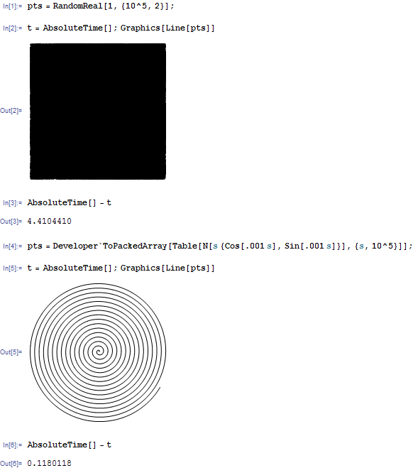
enter image description here

The same number of points, but the rendering of the second one is much faster.

Now, back to our problem. When we are using ListLinePlot without any options (or just PlotRange->All), the process is very close to what Leonid's myListPlot is doing. Which means that it will generate a long chain of Line[{pt1, pt2, ...}] and the self-intersection routine will kick in. If you see the original result closely, you will see that in fact, the resulting graphics has a lot of self-intersection in pixel-res space (it does computation on pixel-level).

Solutions

In fact, Mr.Thomas already got his own answers.

  1. Turing off anti-aliasing (by Style[..., AntiAliasing->False]). This way, the rasterizer spend a lot less time processing intersections, thus much much faster.

  2. Sub-sampling. There are multiple ways, MaxPlotPoints is one, Thomas' code is another, and much more.

  3. Cheating by making multiple paths:

Well, this solution isn't going to give you super boost. Just in case you absolutely need anti-aliasing, and also need to use all the points. Look at a part of my first example:

Line[Partition[pts, 2, 1]]

You will see that we are essentially turning Line[{pt1, pt2, pt3, pt4, ...}] into Line[{{{pt1, pt2}}, {{pt2, pt3}}, {{pt3, pt4}}, ...}]. As long as the opacity remains 1, the result should be about the same (except JoinedForm, but in our case it is no concern). The benefit of the second form is that now it is not considered to be a single path. So, the rasterizer will think that it is multiple-path, and no self-intersection treatment.

I modified Lenoid's myListPlot a bit so that it does this task.

ClearAll[myListPlot2];
Options[myListPlot2] = {AspectRatio -> GoldenRatio^(-1), Axes -> True,
    AxesOrigin -> {0, 0}, PlotRange -> {All, All}, 
   PlotRangeClipping -> True, 
   PlotRangePadding -> {Automatic, Automatic}};

myListPlot2[pts_List, opts : OptionsPattern[]] :=
 Module[{pts1, pts2},
  pts1 = Developer`ToPackedArray@
    Transpose[{N@Range[Length[pts]], pts}];
  pts2 = Partition[pts1, 2, 1];
  Graphics[{{{}, {}, {Hue[0.67, 0.6, 0.6], Line[pts2]}}}, 
   FilterRules[{opts, Options[myListPlot]}, Options[Graphics]]]]

Now, time to prove the theory. With the same data set rv, here is the timing comparison between myListPlot and myListPlot2 (myListPlot is faster than ListLinePlot so it is enough).
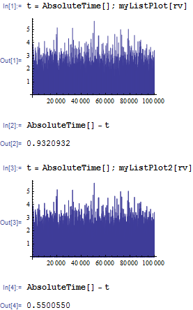
enter image description here

Well, about twice as fast. Frankly, it is not that practical, just theoretical interest :)

Addendum

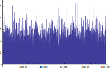
Szabolcs found some bundling going on at 500 (Not sure it is Windows specific or number is exactly that, but bundling is true), which makes me experimenting with different segmenting--instead of just 2, partitioning it at 3, 4, ... etc. And I got all different speed result (getting faster, then slower again). If you use Partition it drops the tail (and I personally am still learning all complex syntax, so...), but it shouldn't make that much of difference, in my opinion.

So, the problem is probably not just affected by the self-intersection, but also the bundling. It gets more interesting / complex :)
$\endgroup$
11
  • 4
    $\begingroup$ Somehow this got cut off. BTW I'm also suffering from slow line-drawing speed right now, and I found that in my application (some generative art experimentation), more than 50% of the time is spent in ToBoxes, not in actual rendering. Strangely, using something like graphicsExpr /. Dispatch[{Graphics -> GraphicsBox, Line -> LineBox}], etc., can be near-instantaneous while ToBoxes can take more than 10 seconds for the same input. I'm wondering if ToBoxes really needs to be so slow, or maybe there's a bug that causes a performance problem? $\endgroup$
    – Szabolcs
    Commented May 10, 2012 at 8:10
  • 4
    $\begingroup$ Very cool and informative - big +1. $\endgroup$ Commented May 10, 2012 at 9:03
  • 1
    $\begingroup$ I experimented a little bit with this. I noticed that something like Graphics[{Thick, Opacity[0.2], Line@Accumulate@RandomReal[{-1, 1}, {10000, 2}]}] does get darker as the line gets longer. It seems that a line "start to overlap itself" after 500 points. Manipulate[ Graphics[{Opacity[0.3], Thickness[0.1], Line[Sequence @@@ Table[{{0, 0}, {1, 1}, {1, 0}, {0, 1}}, {i}]]}], {i, 1, 500}] I wonder if this is system-dependent or not. Is it Mathematica that breaks the link into 500-point segments before passing it to the OS or it's GDI+ that's doing this. $\endgroup$
    – Szabolcs
    Commented May 10, 2012 at 10:42
  • 3
    $\begingroup$ Instead of Partition[Riffle[pts1, Rest[pts1]], 2] you could use the simpler Partition[pts1, 2, 1]. $\endgroup$
    – celtschk
    Commented May 10, 2012 at 10:56
  • 2
    $\begingroup$ To avoid losing the final points for larger partitions, you can use the extra arguments 1,{}, e.g. Partition[pts1,20,19,1,{}]. $\endgroup$
    – celtschk
    Commented May 11, 2012 at 7:57
25
$\begingroup$

Short version

Use Interpolation.

Long version

My fire-and-forget approach to this is interpolating the data first and then plotting it, which is (much to my surprise) orders of magnitudes faster than directly plotting the dataset.

In general, ListPlot and friends really plot the whole list, they make no selection of points. A million points dataset will produce a million plotted points (and then some, consider connecting them with lines etc).

Let's have a look at an example, plotting $\sin(x)\sin(x\,y)$. For eyecandy, this is what it looks like:

Plot3D[Sin[x] Sin[x y], {x, -\[Pi], \[Pi]}, {y, -\[Pi], \[Pi]}, MaxRecursion -> 5, PlotPoints -> 64]

Direct plot of sin(x)sin(xy)

Let's generate the corresponding dataset, a list with entries of the form $\bigl(x, y, f(x, y)\bigr)$.

step = .1;
data = Table[{x, y, Sin[x] Sin[x y]}, {x, -3, 3, step}, {y, -3, 3, step}] // Flatten[#, 1] &;

Now let's compare the plot performance of this dataset, once directly given to ListPlot3D, and then first converted to an InterpolatingFunction via Interpolation[data], and then plotted as a continuous function using Plot3D.

First@AbsoluteTiming[ListPlot3D[data]]
4.220737 seconds
First@AbsoluteTiming[ListPlot3D[data, MaxPlotPoints -> 32]]
17.555031
First@Timing[
    interpolation = Interpolation[data];
    Plot3D[interpolation[x, y], {x, -3, 3}, {y, -3, 3}]
]
0.182330 seconds
First@Timing[
    interpolation = Interpolation[data];
    Plot3D[interpolation[x, y], {x, -3, 3}, {y, -3, 3}, PlotPoints -> 32]
]
0.426254 seconds

As you can see, the interpolated version is faster by over an order of magnitude. In practical use, this method has two shorcomings, however, these can easily be resolved:

  1. You have to specify the data range for the Plot function yourself, as the InterpolatingFunction generated by Interpolation doesn't explicitly show its range. Solution: This information can easily be extracted from the InterpolatingFunction object via Part ("double brackets"): interpolation[[1]] yields {{-3., 3.}, {-3., 3.}}, which is of the form {{xMin, xMax},{yMin, yMax}}.

  2. The plot is of lower quality than the original dataset, since smoothing etc. is done automatically. To solve this general problem, use PlotPoints and MaxRecursion as usual.

Solution, ready to copy+paste

FastListPlot[data_,opts:OptionsPattern[]]:=Module[
    {interp},

    interp=Interpolation[data];
    Plot[interp[x],{x,interp[[1,1,1]],interp[[1,1,2]]},opts]
]
FastListPlot3D[data_,opts:OptionsPattern[]]:=Module[
    {interp},

    interp=Interpolation[data];
    Plot3D[
        interp[x,y],
        {x,interp[[1,1,1]],interp[[1,1,2]]},
        {y,interp[[1,2,1]],interp[[1,2,2]]},
        opts
    ]
]
$\endgroup$
10
  • $\begingroup$ This downsamples, but it does not avoid aliasing effects. Instead one could just use MaxPlotPoints for downsampling. You can look at the original thread Thomas is linking to to understand what the problem is and why this doesn't solve it. (In short: if there are outliers / rare large values in the data, this approach will still effectively filter them out) $\endgroup$
    – Szabolcs
    Commented Jan 25, 2012 at 20:28
  • $\begingroup$ Copying my example from the comments there (which is btw included by the OP too): rv = RandomVariate[ExponentialDistribution[2], 10000]; if = ListInterpolation[rv]; {min, max} = First@if["Domain"] Then compare Plot[if[x], {x, min, max}, PlotRange -> All] and ListLinePlot[rv, PlotRange -> All]. They look strikingly different, i.e. your method does not preserve the shape of the data nearly as well as the OP's method. $\endgroup$
    – Szabolcs
    Commented Jan 25, 2012 at 20:32
  • $\begingroup$ I have to disagree with your first post: Downsampling with MaxPlotPoints makes things much worse on my computer. $\endgroup$
    – David
    Commented Jan 26, 2012 at 5:00
  • $\begingroup$ I could make your version FastListPlot to look like the original ListLinePlot by using 2 changes: Use InterpolationOrder->0 in the definition (otherwise: one gets artifacts close to the x-axis for the particular data set rv defined in the OP), and, in the Plot itself, go up to MaxRecursion->11. This last step, however, made it very slow, slower than the original ListLinePlot. There might be more appropriate options for Plot than MaxRecursion to achieve better sampling, but I haven't tried. $\endgroup$
    – Thomas
    Commented Jan 26, 2012 at 10:29
  • $\begingroup$ @Thomas That's a situational option that depends on the data set. You can still set those options manually when using FastListPlot as you would for other plots. $\endgroup$
    – David
    Commented Jan 26, 2012 at 15:45
22
$\begingroup$

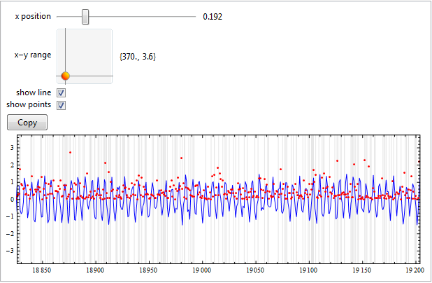
This might not answer all the speed-problems, but it is my solution to plot enormous datasets. By using a dynamic interface it is possible to only show (and keep in memory(?)) a small range of the whole plot, which makes visual analysis of and interaction with the plot much more fluid. The key point is to only update the PlotRange dynamically and not the entire plot.

It works nicely even when downsampling/interpolation is not possible, because e.g. each datapoint must be plotted. Both horizontal and vertical ranges can be set, and I also added some other functionality to test that it works as expected.

(* number of datapoints and some random datasets *)
n = 10^5;
lineData = Table[Sin[x] + RandomReal@{-.5, .5}, {x, 0, n, 1}]; 
pointData = RandomVariate[ExponentialDistribution@2, n];
timeData = RandomInteger[{0, n}, n/2];

DynamicModule[{plot, window = 0, range = {100, 2}, showLine = True, 
  showPoints = True},
 Panel@Grid[{
    {"x position", Row@{Slider@Dynamic@window, Spacer@10, Dynamic@window}},
    {"x-y range", Row@{Slider2D[Dynamic@range, {{100, 1}, {3000, 30}}], Spacer@10, Dynamic@range}},
    {"show line", Checkbox@Dynamic@showLine},
    {"show points", Checkbox@Dynamic@showPoints},
    {Item[Dynamic@Button["Copy", CopyToClipboard@plot, ImageSize -> 60], 
      Alignment -> Left], SpanFromLeft},
    {Item[Dynamic[plot = Show[
         If[showLine, 
          ListPlot[lineData, Joined -> True, PlotStyle -> Blue, 
           PlotRange -> All], Graphics@{}],
         If[showPoints, 
          ListPlot[pointData, Joined -> False, PlotStyle -> Red, 
           PlotRange -> All], Graphics@{}],
         ImageSize -> {600, 200}, AspectRatio -> Full, Frame -> True, Axes -> False,
         PlotRange -> 
          Dynamic@{{Max[n*window - range[[1]], 0], 
             Max[n*window, range[[1]]]}, {-range[[2]], range[[2]]}},
         PlotRangePadding -> {[email protected], [email protected]}, 
         GridLines -> {timeData, {}}, GridLinesStyle -> [email protected]],
       TrackedSymbols :> {showLine, showPoints}], Alignment -> Left], 
     SpanFromLeft}
    }, Alignment -> {{Right, Left, Left}, Center}]]

Mathematica graphics

$\endgroup$
1
  • 1
    $\begingroup$ +1 This should be the answer. You have "quality" and "interpretability" first and foremost. $\endgroup$
    – JimB
    Commented May 14, 2017 at 19:47
19
$\begingroup$

This will work low-level and produce a mostly equivalent plot, but be quite a bit faster:

ClearAll[myListPlot];
Options[myListPlot] = {
   AspectRatio -> GoldenRatio^(-1), Axes -> True, 
   AxesOrigin -> {0, 0}, 
   PlotRange -> {All, All}, PlotRangeClipping -> True, 
   PlotRangePadding -> {Automatic, Automatic}
};
myListPlot[pts_List, opts : OptionsPattern[]] :=
Graphics[{{{}, {}, {Hue[0.67, 0.6, 0.6],
  Line[
    Developer`ToPackedArray@
      Transpose[{N@Range[Length[pts]], pts}]]}}}, 
  FilterRules[{opts, Options[myListPlot]}, Options[Graphics]]]

For example:

In[249]:= rv=RandomVariate[ExponentialDistribution[2],10^5];

In[250]:= (im1=myListPlot[rv]);//AbsoluteTiming
Out[250]= {0.0029296,Null}

In[251]:= t=AbsoluteTime[];im2=ListLinePlot[rv,PlotRange->All];
AbsoluteTime[]-t

Out[252]= 0.4423828

In[253]:= 
(im1/. (AxesOrigin ->_):>AxesOrigin ->First[Cases[im2,(AxesOrigin-> x_):>x,Infinity]])===im2
Out[253]= True
$\endgroup$
2
  • 7
    $\begingroup$ The speed bottleneck really seems to be the rendering. For comparison: on my machine I get: Original ListLinePLot: 1.78 sec; Your myListPlot: 1.4 sec; my fastListPlot: 0.18 sec $\endgroup$
    – Thomas
    Commented Jan 18, 2012 at 14:47
  • $\begingroup$ @Thomas Oh I see. I was suppressing the output and therefore did not observe this. You must be right. Was worth a try, anyways. $\endgroup$ Commented Jan 18, 2012 at 15:13
12
$\begingroup$

My own solution:

Note: I have earlier posted this answer as part of the question itself. I have now removed it there and put it as independent answer.

(see also here for a simpler version of this)

Options[fastListPlot] = {plotPoints -> 1000, AspectRatio -> Full, PlotRange -> All, Options[ListLinePlot]} // Flatten;
fastListPlot[data_, opts:OptionsPattern[]] := 
    Module[{plotData=data, lengths, range = Automatic, points = OptionValue[plotPoints]},
        While[Depth[plotData] <= 2, plotData= {plotData}];
        lengths = Length/@plotData;
        If[NumericQ[points],
           plotData = Partition[#, Floor[Min[lengths]/points]]& /@ plotData;
           plotData = Flatten[{Min /@ #, Max /@ #}\[Transpose]] & /@ plotData;
           range = {1, Max[lengths]}
                   ];
        ListLinePlot[plotData, FilterRules[{opts, DataRange -> range,Options[fastListPlot]},Options[ListLinePlot]]
        ]
    ]

The trick is within the If statement: I partition the data into a number of blocks corresponding roughly to the resolution of my screen (usually 1000 or less, option plotPoints). Then I determine the Min and Max of each block, and draw a zig-zag line from min to max to min to max...

My solution, as presented, works for simple lists (i.e. of Depth 2), and also for lists containing more than 1 data set (Depth 3).

Examples:

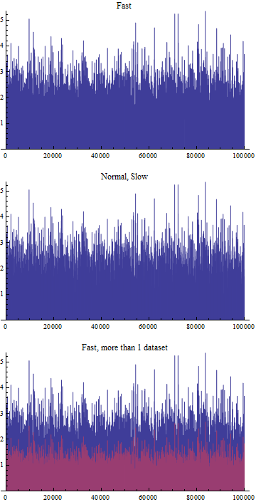
fastListPlot[rv, PlotLabel -> "Fast"]
fastListPlot[rv, plotPoints -> All, PlotLabel -> "Normal, Slow"] 
fastListPlot[{rv,rv/2}, PlotLabel -> "Fast, more than 1 dataset"] 

Mathematica graphics

So, very nicely, the visual structure of the data is preserved, in particular the peaks in the data are preserved and still visible - despite only plotting 2000 points (first plot) instead of 100.000 points (middle plot).

The following doesn't quite work correctly (problem with DataRange):

fastListPlot[{rv,Take[rv/2,10000]}, plotPoints -> All, PlotLabel->"Original"]
fastListPlot[{rv,Take[rv/2,10000]}, plotPoints -> 1000, PlotLabel -> "Incorrect scaling"]

Mathematica graphics

$\endgroup$

Your Answer

By clicking “Post Your Answer”, you agree to our terms of service and acknowledge you have read our privacy policy.

Not the answer you're looking for? Browse other questions tagged or ask your own question.