show a trajectory of a projectile by position vector and velocity vector

Question

We are so motivated to show the projectile motion but emphasize to vector algebra. We could find some help in SE for the projectile motion but non of them have been satisfied our aims. Please see the bellow equation for the position and velocity vectors:

r[t_] := 
  ( v0 Cos[α] t + x0) i +
   0.5 a t^2 + v0 Sin[α] t + y0) j; 
v[t_] := 
  ( v0 Cos[α]) i + (0.5a t + v0 Sin[α] t) j

in which the arbitrary parameters (a<0, v0, α, x0, y0) can be defined before running. In an explicit format

The parabolic shape of the projectile can be given by:

y[x_] := 
  (a x^2)/(2 v0^2 Cos[α]^2) + x Tan[α] + y0

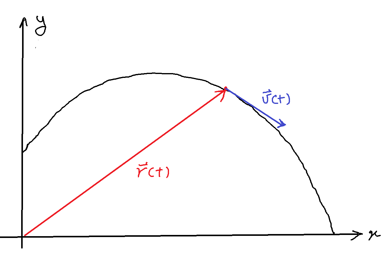
Firstly we wish to have a figure containing the position and velocity vector as functions of time and should be animated by Manipulate function. Same as:

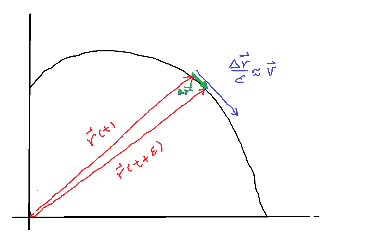
Secondly, it is very interesting to have the approximate velocity obtained from Δr/ϵ, in which ϵ can be changeable, and the real velocity for getting better comparison between them. They are plotted in the bellow figure

Answer 1

Keeping it simple...

Define parameters

a = -10; v0 = 5; α = Pi/4; x0 = 0; y0 = 3;

Express position and velocity explicitly as vectors using List

r[t_] := {v0 Cos[α] t + x0, 0.5 a t^2 + v0 Sin[α] t + y0}
v[t_] := {v0 Cos[α], a t + v0 Sin[α]}

Plot the trajectory

traj = ParametricPlot[r[t], {t, 0, 1.2}, PlotStyle -> Black]

Define functions to display arrows

rvec[t_] := Arrow[{{0, 0}, r[t]}]
vvec[t_, ϵ_] := Arrow[{r[t], r[t] + ϵ v[t]}]
avec[t_, ϵ_] := Arrow[{r[t], r[t + ϵ]}]

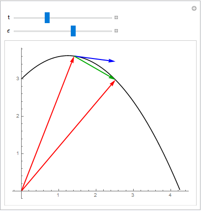
Show all the graphics and Manipulate t, ϵ

Manipulate[Show[traj, Graphics[{Thick,
    Red, rvec[t], rvec[t + ϵ], Blue, vvec[t, ϵ], Darker[Green], avec[t, ϵ]}]],
 {t, 0, 1.2}, {ϵ, 0.01, 0.5}]

Answer 2

It is possible, and likely instructive, to generate the equations from a more general starting point. The following is not yet completely general due to the assumption of constant accelerations ax and ay, but further generalization is easily implemented. Also, you can just Integrate to recover the explicit formulas if you wish.

eqnDefs = {
r''[t] == {ax, ay},
r'[0] == {v0 Cos[𝛼0], v0 Sin[𝛼0]},
r[0] == {x0, y0}
} 
/. {ax -> 0, ay -> -9.81, v0 -> 20, 𝛼0 -> π/3, x0 -> 0, y0 -> 0}

Then you just numerically solve the differential equations with NDSolve

soln = First@NDSolve[
eqnDefs,
{r},
{t, 0, 10}
]

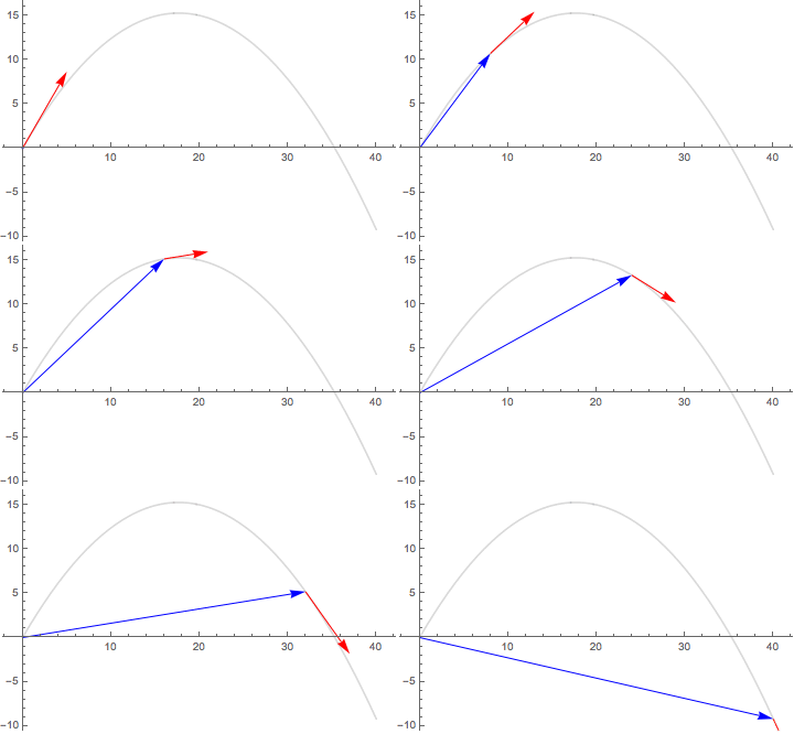
Finally, you use ParametricPlot to show the trajectory and Graphics to generate the vector depictions using Arrow.

Manipulate[
 Show[{ParametricPlot[
    Evaluate[r[tt] /. soln],
    {tt, 0, 4},
    PlotStyle -> Directive[Opacity[.3], Gray]
    ],
   Graphics[
    {Blue, Arrow[{{0, 0}, r[t] /. soln}],
     Red, 
     Arrow[{r[t] /. soln, 
       Evaluate[r[t] /. soln ] + Evaluate[ r'[t] /. soln]/2}]
     }]    
   }],
 {{t, 2}, 0, 4}
]

Answer 3

There are a number of issues. The equations are not correct (they are dimensionally inconsistent). In the following the acceleration is taken as 9.8 $\text{m}\cdot\text{s}^{-2}$:

Simple equation of motion:

r[v0_, a_, y0_, t_] := {0, -4.9 t^2} + v0 t {Cos[a], Sin[a]} + {0, y0}

Calculating time and x position that $y(t)=0$:

hit[v0_, a_, y0_] := 
  Quiet[{u, x} /. 
    Solve[r[v0, a, y0, u] == {x, 0} && u > 0, {u, x}][[1]]];

Calculate peak of trajectory:

pk[v0_, a_, y0_] := 
  r[v0, a, y0, t] /. 
   Quiet[Solve[D[r[v0, a, y0, t], t][[2]] == 0, {x, t}][[1]]];

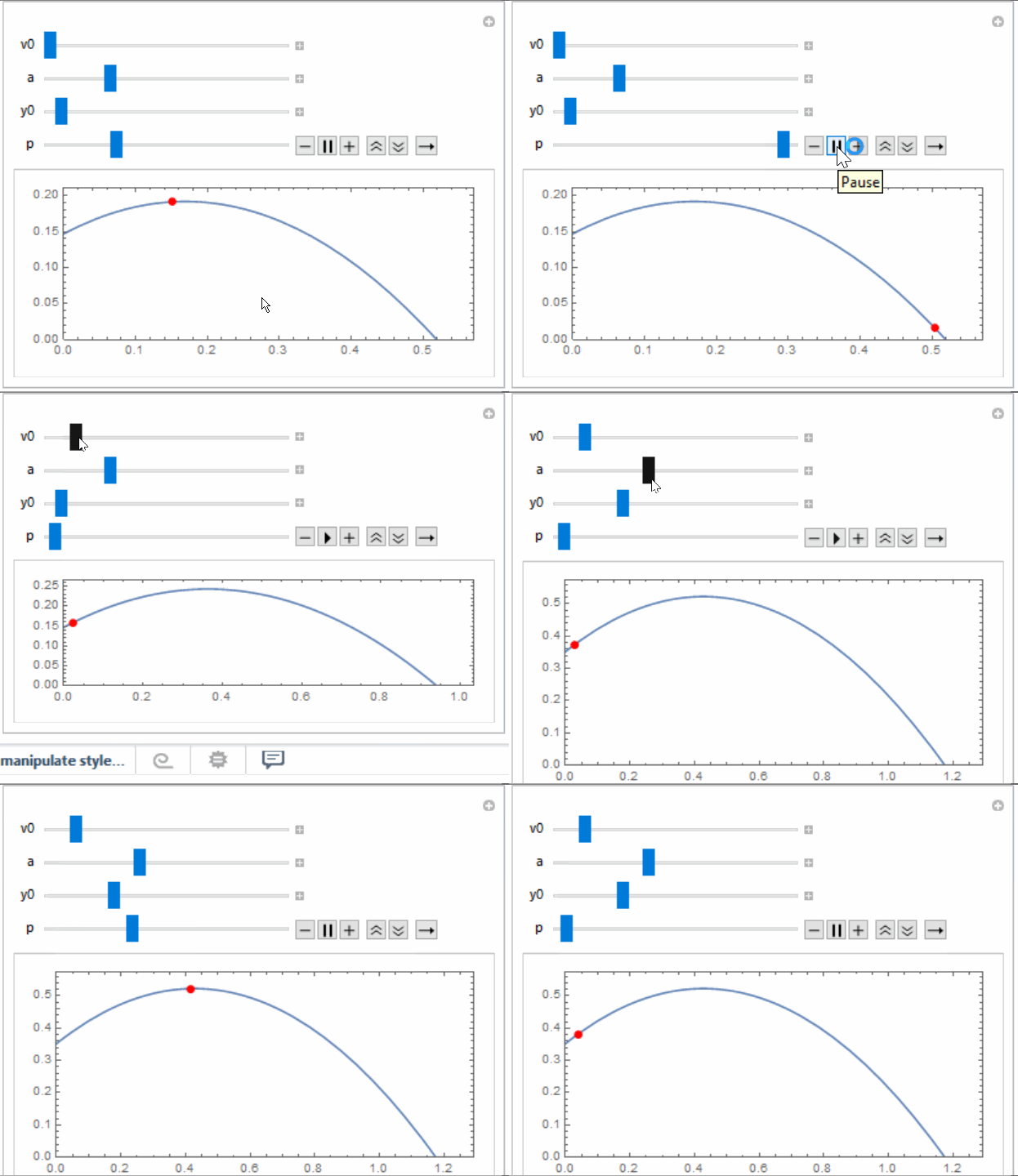
A function to allow visualization:

func[v0_, a_, y0_, p_] := Module[{xh, th, peak = pk[v0, a, y0][[2]]},
  {th, xh} = hit[v0, a, y0];
  ParametricPlot[r[v0, a, y0, t], {t, 0, th}, 
   PlotRange -> {{0, 1.1 xh}, {0, 1.1 peak}}, 
   Epilog -> {Red, PointSize[0.02], Point[r[v0, a, y0, p th]]}, 
   Frame -> True]]

Visualizing:

Manipulate[
 func[v0, a, y0, p], {v0, 2, 10}, {{a, 1}, 0.1, Pi/2}, {y0, 0.1, 
  1}, {p, 0, 1, Animator}]