ListLinePlot with vertical filling gradient

Question

I am aware that the topic of vertical filling has been discussed before (e.g., here and here), but I could not find any reasonably simple solution to the following problem:

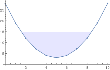
I have a discrete data set which I plot with ListLinePlot. I want to fill the area between the data and a given y value if the data is below that value. That much is easy:

data = Table[{x, (x - 5)^2 + 3}, {x, 0, 10}];

Show[ListLinePlot[data, 
  Filling -> {1 -> {15, {Directive[Blue, Opacity[0.1]], None}}}], 
 ListPlot[data]]

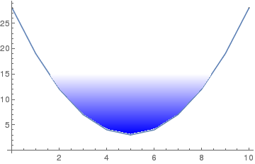
However, now I want the filling to have a vertical gradient in opacity (or white level, I don't really mind) such that the filling is blue at y=3 and transparent for y>15. I found a solution for filling under all data points using polygons and for parametrizable functions. However, as it happens, my filling does not end at a data point and it seems to me that applying the polygon solution would be quite a hack that involves first finding and constructing proper boundary points for the polygon.

Is there really no simpler way for vertical gradients?

Edit:

Just for the sake of completeness, I realized that the above link (filling under all data points) does give a suggestion of how to use ParametricPlot together with Interpolate to create a vertical gradient filling on discrete data. The code would look like this:

interp = Interpolation[data, InterpolationOrder -> 1];
Show[ListLinePlot[data], 
 ParametricPlot[{x, 
   With[{value = 15 (1 - y) + interp[x] y}, 
    If[value > interp[x], value]]}, {x, 0, 10}, {y, 0, 1}, 
  ColorFunction -> (Blend[{Blue, White}, #2] &), 
  BoundaryStyle -> None]]

However, the result is much less appealing then the polygon solution. It is possible to improve the quality by ramping up the PlotPoints, but then it takes very long to calculate the graph and exporting it, in particular to pdf, crashes Mathematica completely on my computer.

Answer 1

As you say, it's a hack, but it's a relatively small one:

p1 = ListLinePlot[data, Filling -> {1 -> {15, {Blue, None}}}, PlotMarkers -> Automatic]

(I changed the Filling parameters on a suggestion by the OP.)

Then:

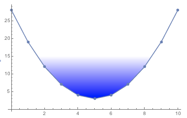
Normal@p1 /. Polygon[x_] :> Polygon[x, VertexColors -> (Blend[{Blue, White}, #] & /@ Rescale[x[[All, 2]]])]

The Rescale stuff is meant to re-scale the y-values so that they go between 0 and 1, allowing us to Blend from Blue to White. (Thanks to MarcoB for the nicer code.)

Answer 2

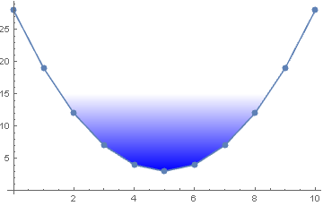
Using LinearGradientFilling: (Introduced with v12.2, 2020)

data = Table[{x, (x - 5)^2 + 3}, {x, 0, 10}];

ListLinePlot[data
 , Mesh -> All
 , Filling -> {1 -> {15, {Directive[
       LinearGradientFilling[{Blue, White}, Top]]
      , None
      }
     }
   }
 ]

---