Displace the origin of a function plot with respect to another function

Question

thank you for your explainations. Both of the proposed solutions:

Plot[g[x - a] - g[0] + f[a], {x, a, a+b}] by Michael E2
f3[x_] := Piecewise[{{f1[x], 0 <= x<= 5}, {f2[x - 5], 5 < x <= 20}}] by m_goldberg

look to be promising but as the real problem is a little more complicated and being a newbie with mathematica, I'll try to be more specific. I want to draw light propagation inside an optical system by using ABCD matrices. As an example, I define three matrices m6,m7 and m8

m6 = {{1, x}, {0, 1}}; 
m7 = {{1, 0}, {-1/f, 1}}; 
m8 = {{1, ldl}, {0, 1}}; 

where x and ldl are distances and f is a fixed numerical value for a lens power.

I use these numerical values:

y0 = 10 10^-6;
t0 = 0 Pi/180;
f = 50 10^-3;
ldlt = 10 10^-2;
xt = 30 10^-2;

Then I want to plot the trends of y1 and y2 given by

{y1, t1} = m8.{y0, t0} 
y1t = Table[y1, {ldl, 0, ldlt, ldlt/100 }];
t1t = Table[t1, {ldl, 0, ldlt, ldlt/100 }];
{y2, t2} = m6.m7.{y1t[[101]], t1t[[101]]}. 

y1t and t1t are the last values of y0 and t0 vectors. I tried with

Show[Plot[y1, {ldl, 0, ldlt}], Plot[y2, {x, 0, xt}]] 

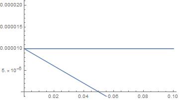
to plot both of them but doing like this, y2 (the inclined line) will always start from the origin and not from the last point of y1 (0.1 in the attached graph).

Then, each matrix will use a different name for the spatial variable, so for me, x is reserved to a parameter that I want to optimize; I have 20 matrices like this in the code.

So the problem is how to make each plot start from the end of the previous one ideally by keeping the proper spatial variable name (ldl, x, whatever).

Thank you for any help

Answer 1

I am not sure I understand your question, but perhaps you are looking for Piecewise.

Consider

f1[x_] := 5 - x
f2[x_] := Sqrt[x]

and let's combine them with Piecewise.

f3[x_] := Piecewise[{{f1[x], 0 <= x<= 5}, {f2[x - 5], 5 < x <= 20}}]

then

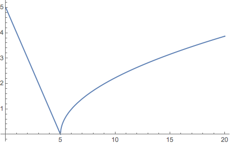
Plot[f3[x], {x, 0, 20}]

Does this work for you?

Answer 2

Update: A function to concatenate several plots:

ClearAll[displaceF]
displaceF[p__Graphics] := Module[{d = Accumulate[PlotRange[#][[1, 2]]&/@ Most[{p}]]},
  Show[{p}[[1]], Graphics[Translate[#[[1]], {#2, 0}] & @@@ Transpose[{Rest@{p}, d}]], 
   PlotRange -> All]]

Example:

f1[x_] := Sin[x] + Sin[Sqrt[2] x]
f2[x_] := x Cos[Sqrt[2] x] 
f3[x_] := (4 Pi - x) Cos[4 Pi - x]

plt1 = Plot[f1[x], {x, 0, 10 Pi}, PlotStyle -> Green];
plt2 = Plot[f2[x], {x, 0, 4 Pi}, PlotStyle -> Red];
plt3 = Plot[f3[x], {x, 0, 4 Pi}, PlotStyle -> Blue];

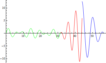
displaceF[plt1, plt2, plt3]

Original post:

Maybe you can use Translate as follows:

f1[x_] := Sin[x]
f2[x_] := x Cos[x]

Show[Plot[f1[x], {x, 0, 2 Pi}, PlotStyle -> Green], 
 Graphics[Translate[Plot[f2[x], {x, 0, 4 Pi}, PlotStyle -> Red][[1]], {2 Pi, 0}]], 
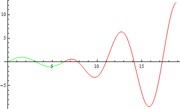
 PlotRange -> All]

Alternatively, you can use the translated graphics primitives of the second plot as Epilog in a plotting the first function:

Plot[f1[x], {x, 0, 2 Pi}, PlotStyle -> Green, 
 Epilog -> Translate[Plot[f2[x], {x, 0, 4 Pi}, PlotStyle -> Red][[1]], {2 Pi, 0}], 
 PlotRange -> {{0, 6 Pi}, {-10, 10}}]