Wonky Solutions to Schrödinger Equation with Box Barrier

Question

I'm trying to solve the Schrödinger equation using NDSolve in a case where there is a potential box barrier. The initial condition is a cosine wave, and for boundary conditions I require that the solution on the ends of domain is 0. Essentially I am encapsulating a potential barrier within infinite walls. (I am also hoping this requirement allows for reflections off the walls.) I'm getting a solution that oscillates but it doesn't behave like what I would expect. Increasing the barrier size I expect the wavefunction to go to 0 within the barrier, but instead the oscillations that happen in the barrier are more frequent the larger the barrier. This doesn't make sense, and I don't know of a different way of solving the equation in Mathematica.

My code is this:

ClearAll["Global`*"]
e = 1; (* energy *)
k1[e_] = Sqrt[2 e];

s = NSolve[Cos[k1[e] x] == 0, x, WorkingPrecision -> 16];
L = N[s[[1, 1, 2, 1]] /. C[1] -> -5, 16] (* left boundary *)
R = N[s[[1, 1, 2, 1]] /. C[1] -> 5, 16] (* right boundary *)

width = 2; (* potential height and width *)
height = 2;
a = 1/Sqrt[Integrate[(Cos[k1[e] x])^2, {x, L, R}]]; (* normalization of input *)

eqn = D[ψ[x, t], t] == 
I/2 D[ψ[x, t], {x, 2}] - 
I*ψ[x, 
  t]*(Piecewise[{{0, x <= 0}, {height, 0 < x < width}, {0, 
     x >= width}}]);

bc = {ψ[L, t] == 0, ψ[R, t] == 0};

ic = {ψ[x, 0.] == a Cos[k1[e] x]};

sol = NDSolve[{eqn, bc, ic}, ψ, {x, L, R}, {t, 0, 20}, 
Method -> {"MethodOfLines", 
"SpatialDiscretization" -> {"TensorProductGrid", 
"DifferenceOrder" -> "Pseudospectral"}}, AccuracyGoal -> 10, 
PrecisionGoal -> 10]

Manipulate[
Plot[{Re[ψ[x, t] /. sol], 
Piecewise[{{0, x <= 0}, {height, 0 < x < width}, {0, 
x >= width}}]}, {x, L, R}, PlotRange -> {-2, 3}], {t, 0, 20, 
0.1}]

I'm using Mathematica 11 on Linux. Any help or direction is appreciated.

Edit: Complex valued 2+1D PDE Schrödinger equation, numerical method for `NDSolve`? This is a similar post, and one of the answers implements Dirichlet boundary conditions. I'm having trouble understanding how the boundary conditions were constructed but they are probably important to solving my problem.

Answer 1

This problem can be solved quite quickly and accurately by computing its eigenfunctions, projecting the initial condition onto the eigenfunctions, and then summing them. With parameters,

e = 1; k1[e_] = Sqrt[2 e];L = -(2 Pi + Pi/2)/ k1[e]; R = (2 Pi - Pi/2)/ k1[e]; 
    w = 2; a = 1/Sqrt[(R - L)/ k1[e]]; ic = a Cos[k1[e] x]

the solution is given by

ss[hh_, t_] := 
  Module[{ms, mc, op = - D[ψ[x], {x, 2}]/2 + ψ[x]*Piecewise[{{hh, 0 < x < w}}, 0]}, 
    ms = NDEigensystem[{op, DirichletCondition[ψ[x] == 0, True]}, ψ[x], {x, L, R}, 30, 
      Method -> {"SpatialDiscretization" -> {"FiniteElement", 
      {"MeshOptions" -> {"MaxCellMeasure" -> (R - L)/1000}}}}]; 
    mc = Table[Quiet@NIntegrate[ms[[2, i]] ic, {x, L, R}, 
      Method -> "ClenshawCurtisRule", MaxRecursion -> 18], {i, 30}]; 
    mc.(Exp[-I First@# t] Last@# & /@ Transpose@ms)]

sol[2] = ss[2, 20];
sol[5] = ss[5, 20];
sol[8] = ss[8, 20];
Plot[Evaluate[Re@sol[#] & /@ {2, 5, 8}], {x, L, R}, PlotRange -> 1]

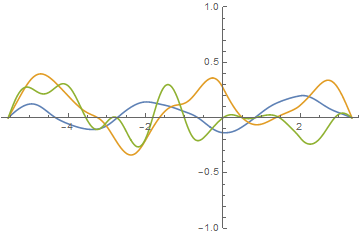
Increasing the number of eigenfunctions (here, 30) or decreasing the MaxCellMeasure (equivalent to about 1000 grid points) has no visible impact on the solution.

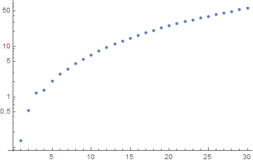
To illustrate the process in more detail, consider h == 2. The eigenvalues (the temporal frequencies of eigenfunctions) and the projection of the initial condition on the eigenfunctions are

ListLogPlot[First@ms]

ListPlot[mc, PlotRange -> All]

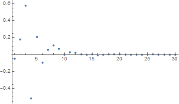
Eigenfunctions 3 and 4 are the primary contributors to the solution. This is so, because their wavelengths are comparable to the wavelength of the initial condition. The first eight eigenfunctions are plotted next.

Plot[Evaluate[ms[[2, 1 ;; 8]]], {x, L, R}, PlotLegends -> Range[8]]

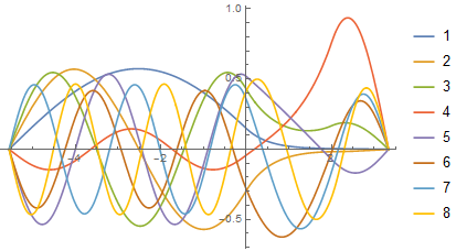
The first three eigenfunctions are restricted mostly to the left of the barrier, because they do not fit in the region to the right of the barrier, although the third shows signs of leaking through. The fourth eigenfunction is quite large in the region to the right of the barrier, probably because a half-wavelength of the eigenfunction matches fairly well the width of the region on the right. (This behavior of eigenfunctions four becomes even more pronounced for larger h.) Higher modes, with frequencies exceeding h penetrate the barrier.

Incidentally, DEigensystem is unable to obtain a symbolic expression for the eigenfunctions, although a symbolic solution does exist and can be obtained using DSolve in each region separately and matching the results across the edges of the barrier. The resulting dispersion function still must be solved numerically.

Addendum

Sample temporal results can be obtained from

sol1[2] = ss[2, t];
sol1[5] = ss[5, t];
sol1[8] = ss[8, t];

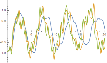
Plot[Evaluate[Re@(sol1[#] /. x -> -2.5) & /@ {2, 5, 8} ], {t, 0, 20}]

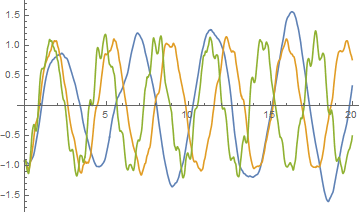
Plot[Evaluate[Re@(sol1[#] /. x -> 2.5) & /@ {2, 5, 8} ], {t, 0, 20}]

Plot[Evaluate[Re@(sol1[#] /. x -> 1) & /@ {2, 5, 8} ], {t, 0, 20}]

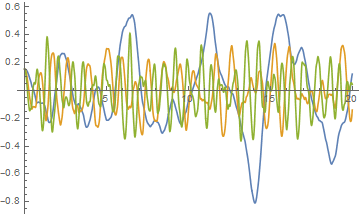
As expected, behavior to the left of the barrier is dominate by the third eigenfunction, to the right by the fourth eigenfunction, and in the barrier by high frequency eigenfunctions that can penetrate the barrier.

Second Addendum - Large Domain

The computation above used a fairly small domain in order to facilitate comparison with the answer by xzczd. The domain presented in the question is substantially larger,

L = -(10 Pi + Pi/2)/ k1[e]; R = (10 Pi - Pi/2)/ k1[e]; 

Results for this case too can be obtained, although doing so requires n == 120 eigenfunctions and Method adjustments to NDEigensystem.

ss[hh_, t_] := 
  Module[{ms, mc, op = - D[ψ[x], {x, 2}]/2 + ψ[x]*Piecewise[{{hh, 0 < x < w}}, 0]}, 
    ms = NDEigensystem[{op, DirichletCondition[ψ[x] == 0, True]}, ψ[x], {x, L, R}, 120, 
    Method -> {"Eigensystem" -> "Arnoldi", "MaxIterations" -> 2000}, 
      "SpatialDiscretization" -> {"FiniteElement", 
        {"MeshOptions" -> {"MaxCellMeasure" -> (R - L)/1000}}}}]; 
    mc = Table[Quiet@NIntegrate[ms[[2, i]] ic, {x, L, R}, 
      Method -> "ClenshawCurtisRule", MaxRecursion -> 30], {i, 120}]; 
    mc.(Exp[-I First@# t] Last@# & /@ Transpose@ms)]

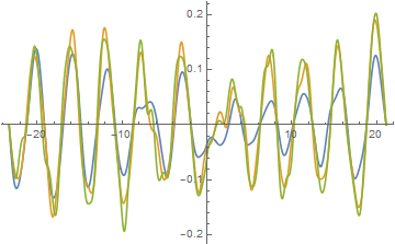
The resulting curves are somewhat different from those above,

Plot[Evaluate[Re@sol[#] & /@ {2, 5, 8}], {x, L, R}]

Because the barrier occupies only about 5% of the computational region, a blowup is helpful.

Plot[Evaluate[Re@sol[#] & /@ {2, 5, 8}], {x, -w, 2 w}]

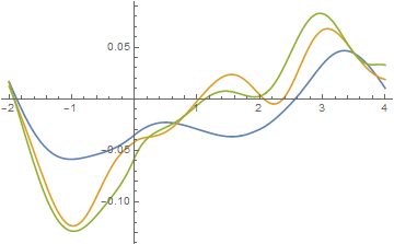
Eigenfunctions in the range 16 - 23 dominate these plots, except inside the barrier, where higher frequency eigenfunctions dominate. Only about 15 minutes was required to compute these two plots.

Answer 2

You can use a appropriate 4th order spatial grid:

e = 1;(*energy*)
k1[e_] = Sqrt[2 e];
s = NSolve[Cos[k1[e] x] == 0, x, WorkingPrecision -> 16];
L = N[s[[1, 1, 2, 1]] /. C[1] -> -1, 16] (*left boundary*)
R = N[s[[1, 1, 2, 1]] /. C[1] -> 1, 16] (*right boundary*)    
a = 1/Sqrt[Integrate[(Cos[k1[e] x])^2, {x, L, R}]];    
bc = {ψ[L, t] == 0, ψ[R, t] == 0};
ic = {ψ[x, 0.] == a Cos[k1[e] x]};    
Clear@eqn;
width = 2;
eqn[height_] := 
  D[ψ[x, t], t] == 
   I/2 D[ψ[x, t], {x, 2}] - 
    I*ψ[x, t]*(Piecewise[{{0, x <= 0}, {height, 0 < x < width}, {0, x >= width}}]);

mol[n_Integer, o_: "Pseudospectral"] := {"MethodOfLines", 
    "SpatialDiscretization" -> {"TensorProductGrid", "MaxPoints" -> n, 
        "MinPoints" -> n, "DifferenceOrder" -> o}}    
showStatus[status_] := 
  LinkWrite[$ParentLink, 
   SetNotebookStatusLine[FrontEnd`EvaluationNotebook[], ToString[status]]];
clearStatus[] := showStatus[""];
opt = EvaluationMonitor :> showStatus["t = " <> ToString[CForm[t]]];    
solfunc[height_, points_, order_: "Pseudospectral", tbegin_: 0] := (clearStatus[]; 
  NDSolveValue[{eqn[height], bc, ic}, ψ, {x, L, R}, {t, tbegin, 20}, 
   Method -> mol[points, order], MaxSteps -> Infinity, opt])

sol[2] = solfunc[2, 550, 4]; // AbsoluteTiming
(* {17.080840, Null} *)
sol[5] = solfunc[5, 550, 4]; // AbsoluteTiming
(* {29.171855, Null} *)   
sol[8] = solfunc[8, 550, 4]; // AbsoluteTiming
(* {54.542178, Null} *)

Plot[sol[#][x, 20] & /@ {2, 5, 8} // Re // Evaluate, {x, L, R}, PlotRange -> 1]

Definition of showStatus is from here.

Remark

To obtain a reasonable result, the grid should be dense enough i.e. points should not be too small. However, it seems that "dense enough grid" isn't the only requirement, for example solfunc[8, 552, 4, 19] will lead to a catastrophically wrong result after a very slow solving process. I'm not sure why this happens.

I think it's relatively clear from the picture that the function value is going to 0 when height gets larger. If you still feel worried, you can check their integration:

NIntegrate[sol[#][x, 20] & /@ {2, 5, 8} // Re // Abs, {x, 0, 2}]
(* {0.245181, 0.176277, 0.0766969} *)