Programmatic approach to HDR photography

Question

Update

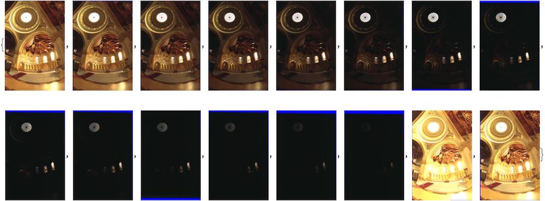
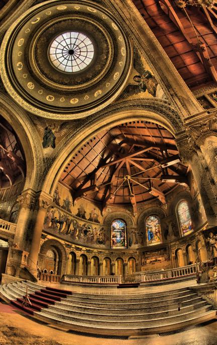
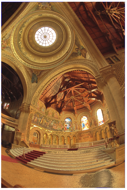
Submitted answers here are tour de force, and very educational comp-sci-wise, -- thanks folks! Tech is developing though, and here is the current implementation in the Wolfram Language. Please study the relevant docs and options of these functions (ImageExposureCombine and ColorToneMapping) and also related functions, for example ImageFocusCombine. So, we got 16 images under different exposures:

imgs=Import["http://www.pauldebevec.com/Research/HDR/SourceImages/Memorial_SourceImages.zip","*.png"];

Thumbnail /@ imgs

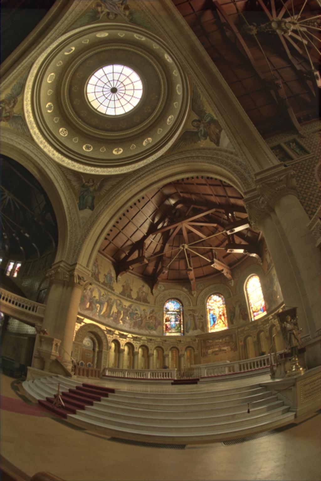
This one-liner does it (with some arbitrary choice of parameters, feel free to experiment):

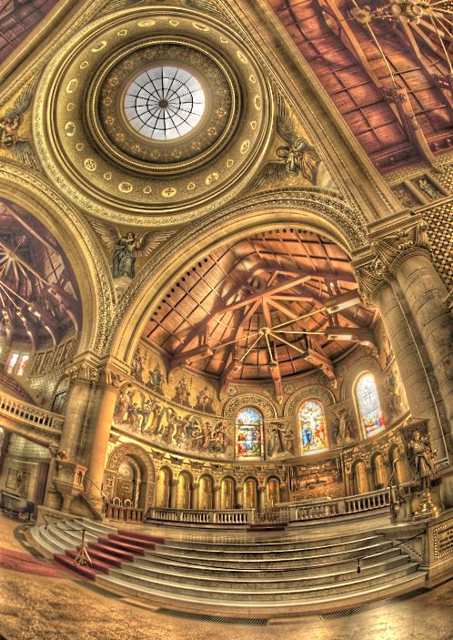
ColorToneMapping[ImageExposureCombine[imgs,"HDR"],.7]

Original post

The High dynamic range imaging (HDR or HDRI) direction in photography and image processing became very popular recently. Besides obvious photo art applications (see examples), there are many great opportunities in computer vision and graphics.The German Max Planck Institute has a page dedicated to the pipeline of related technologies, publications and discussions.

I wonder if our community has members who are knowledgeable enough to reproduce a correct algorithm in Mathematica's top level image processing functions. I hope the answers may also serve as a good intro to methodology from the programmatic point of view. I am sure code will be quite short and consider this to be a very practical down to earth question. There are many Photoshop-like tutorials online. I won't link to them because they are quite easy to find and I cannot judge which one reflects the right approach. Read a concept article about HDR here.

I found this interesting research site with Mathematica notebook and manual provided (read down the page). Unfortunately it gives only part of the process – tone mapping, and is written in Mathematica version 6, while there have been many image processing upgrades in the current version 8.

Precise question formulation:

• Consider a set of images taken at different exposures – like these public images
• Write Mathematica code that produces an HDR image – like the one here labeled “Local tone mapping”
• Implement any HDR algorithm (there are a few) by any Mathematica means possible

Additional resources.

• A review of HDR algorithms

• A classical image set to test an HDR technique is Paul Debevec's HDR photo of Stanford Memorial Church. So I think we can also try to get something like this out of original set of images found on this page.

• This is a related Mathematica.SE question.

Answer 1

Edit.

I have produced an image which is "cleaner" looking than my original attempt, and the processing is faster too.

As before we start by loading the images in order from darkest to brightest, and cropping away the artifacts from alignment.

files = Reverse@FileNames["memorial*.png"];
images = ImagePad[Import[#], {{-2, -12}, {-35, -30}}] & /@ files;

HDR image construction:

Like Thies's approach, this uses averaging over multiple images to obtain pixel values. Intensity data is extracted from the images and low or high values are set to zero to flag potentially noisy or saturated pixels. The exposure ratio between two images is estimated by considering only those pixels which are non-zero in both images. After compensating for exposure differences, the pixel values from all images are combined into a mean image, again using only the non-zero pixels. Finally the mean image is split into HSB components.

data = ImageData[First@ColorSeparate[#, "Intensity"]] & /@ images;
data = Map[Clip[#, {0.1, 0.97}, {0, 0}] &, data, {3}];

exposureratios = Module[{x, A, g}, 
  First@Fit[Cases[Flatten[#, {{2, 3}, {1}}], {Except[0], Except[0]}, 1],
  x, x] & /@ Partition[data, 2, 1]];
exposurecompensation = 1/FoldList[Times, 1, exposureratios];

data = MapThread[Times, {exposurecompensation, Unitize[data] (ImageData /@ images)}];
data = Transpose[data, {3, 1, 2, 4}];
meanimage = Map[Mean[Cases[#, Except[{0., 0., 0.}]]] &, data, {2}];

{h, s, b} = ColorSeparate[ColorConvert[ImageAdjust@Image[meanimage], "RGB"], "HSB"];

Tone mapping:

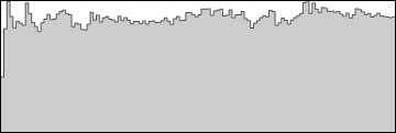
We now have a brightness channel containing a range of values from 0 to 1, but with a very non-uniform distribution.

ImageHistogram[b]

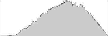
First I do a histogram equalisation on the brightness data:

cdf = Rescale@Accumulate@BinCounts[Flatten@ImageData@b, {0, 1, 0.00025}];
cdffunc = ListInterpolation[cdf, {{0, 1}}];
histeq = Map[cdffunc, ImageData[b], {2}];
ImageHistogram[Image@histeq]

Next I apply a sort of double-sided gamma adjustment to reduce the number of very low and very high values (we don't want too many deep shadow or bright highlights).

b2 = Image[1 - (1 - (histeq^0.25))^0.5];
ImageHistogram[b2]

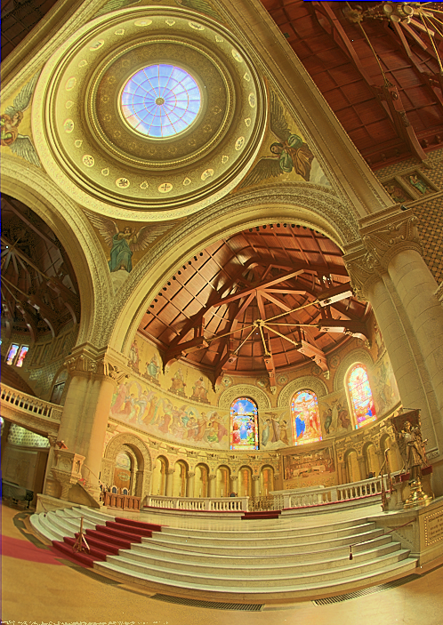
Final image:

Finally I apply a built-in Sharpen filter to the new brightness channel, to boost local contrast a little bit, and apply a gamma adjustment to the saturation channel to make it a little more colourful. The HSB channels are then recombined into the final colour image.

ColorCombine[{h, ImageAdjust[s, {0, 0, 0.75}], Sharpen[b2]}, "HSB"]

Original version

Here's an attempt at the Stanford Memorial Church image using a local contrast filter to do the tone mapping.

First load the images and crop to remove the artifacts around the edges of some of them:

files = Reverse @ FileNames["memorial*.png"];
images = ImagePad[Import[#], -40] & /@ files;

Next create small grayscale versions and use these to estimate the brightness scaling between the images

small = ImageData[ImageResize[ColorConvert[#, "Grayscale"], 50]] & /@ images;
imageratios = FoldList[Times, 1, 
  Table[a /. Last@
    FindMinimum[Total[(small[[i]] - a small[[i + 1]])^2, -1], {a, 1}], 
  {i, Length@small - 1}]]

Now select the "best" image from which to take each pixel value, and scale that value accordingly. I've defined the "best" image for a given pixel as the one for which the median of the {R,G,B} numbers is closest to 0.5.

data = Transpose[ImageData /@ images, {3, 1, 2, 4}];
bestimage = Map[Module[{best},
 best = Ordering[(Median /@ # - 0.5)^2, 1][[1]];
 #[[best]]*imageratios[[best]]] &, data, {2}];

Next apply a local contrast enhancement to the brightness channel of the image. This is quite simple and slow. For each pixel the filter sorts the unique values in the pixel's neighbourhood and finds the pixel's position in that list. The pixel value is set to the fractional list position. For example if a pixel is the brightest one in its neighbourhood, it gets a value of 1. The size value in the localcontrast function must match the range parameter in the ImageFilter.

localcontrast = With[{size = 20}, Compile[{{x, _Real, 2}}, 
Block[{a, b, val}, val = x[[size + 1, size + 1]];
a = Union[Flatten[x]];
b = Position[a, val][[1, 1]];
b/Length[a]]]];

{h, s, b} = ColorSeparate[ColorConvert[Image[bestimage], "RGB"], "HSB"];     
newb = ImageFilter[localcontrast, b, 20];

Finally combine the contrast-enhanced brightness channel with the original saturation and hue to get the final image:

ColorCombine[{h, s, newb}, "HSB"]

It's not brilliant, but I think the general HDRI effect is there. The contrast enhancement could probably be toned down a bit by increasing the size parameter, though it'll be slower.

Answer 2

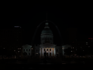
For starters i tried an easy intuitive approach, namely, combining the best parts from each image adjusted for the different exposure times all into one HDR image.

Let's start by importing all the images

imageurls = "http://upload.wikimedia.org/wikipedia/commons/thumb/" <> # & /@
  {"0/09/StLouisArchMultExpEV-4.72.JPG/320px-StLouisArchMultExpEV-4.72.JPG",
   "c/c3/StLouisArchMultExpEV-1.82.JPG/320px-StLouisArchMultExpEV-1.82.JPG", 
   "8/89/StLouisArchMultExpEV%2B1.51.JPG/320px-StLouisArchMultExpEV-1.51.JPG",
   "8/8f/StLouisArchMultExpEV%2B4.09.JPG/320px-StLouisArchMultExpEV-4.09.JPG"};

FPImage = Image[#, "Real"]& (* change image rep. to floating point *)
inputimages = SortBy[
    Composition[FPImage, Import] /@ imageurls,
    (* sort images by increasing exposure *)
    Composition[Mean, Flatten, ImageData, First, ColorSeparate[#, "Intensity"] &]
  ]

where we changed the internal representation to floating point to avoid rounding errors later and already sorted in ascending order by exposure times.

Next we compare neighbour pairs of images and try to guess their exposure ratios. (Probably there is a more robust and effective method, but for first try it seems to work and give reasonably exact values).

ScaledImageSquaredError[img1_Image, img2_Image, s_?NumericQ] :=
  Composition[Total, Flatten, ImageData, ImageApply[#^2 &, #] &,
              First, ColorSeparate[#, "Intensity"] &][
      ImageDifference[img2, ImageClip@ImageApply[s # &, img1]]
    ];

(* Guess exposure ratio. img2 must be the brighter than img1 *)
GuessExposureRatio[img1_Image, img2_Image] := NArgMin[
  {ScaledImageSquaredError[img1, img2, \[Alpha]],
   1 < \[Alpha] < 10},
   \[Alpha], Method -> {"NelderMead", "RandomSeed" -> 24}
]

exposureratios = GuessExposureRatio @@@ Partition[inputimages, 2, 1]
(* {4.66667, 5.89289, 3.74074} *)

(* brightness scaling factors to get all images to the same exposure level *)
unifyingexposures = #/Max[#] &@Reverse@FoldList[Times, 1, Reverse@exposureratios]
(* {1., 0.214286, 0.0363634, 0.00972091} *)

Next we want to generate masks for each image, marking the usable portion of each image. Our criterium will be the brightness of each pixel. We don't want the low-brightness range because of possibly bad signal-to-noise ratios and we don't want the brightnesses near 1.0 because of possible clipped values.

Therefore we define a (kind of arbitrary and adjustable) brightness weight curve

brightnessweights = Function[b, 
    Piecewise[
      {{Interpolation[{{{0}, 0, 0}, {{0.2}, 1, 0}, {{0.95}, 1, 0}, {{1}, 0, 0}},
                      InterpolationOrder -> 3][b],
        0 <= b <= 1}}, 0
    ]
  ]
Plot[brightnessweights[b], {b, 0, 1}, PlotRange -> All, ImageSize -> Small]

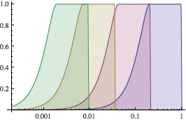
and see how the different exposure regions overlap and combine

LogLinearPlot[
  Evaluate[brightnessweights[b/#] & /@ unifyingexposures],
  {b, 0.0002, 1},
  PlotRange -> All, Filling -> Axis
]

We have good overlap, but not too much, and no gaps in brightness levels, so that looks nice.

Next, we'll construct the weight maps by applying the brightness curve to the brightnesses of each image pixel and then normalizing by the sum of all weight maps at each pixel.

GenerateWeightMask = Composition[
    ImageApply[brightnessweights, #] &, First, ColorSeparate[#, "Intensity"] &
  ]
ImageTotal = Fold[ImageAdd, First@#, Rest@#] &

nrimages = Length[inputimages];
brightnessmasks = GenerateWeightMask /@ inputimages
scaledmasks = ImageMultiply[#, 1/nrimages] & /@ brightnessmasks;
masksum = ImageTotal[scaledmasks];
invmasksum = ImageApply[1/(nrimages #) &, masksum];
weightmasks = ImageMultiply[#, invmasksum] & /@ brightnessmasks

Now we multiply our input images with the weight masks and adjust for the different exposure levels and then combine all those into the final HDR composite image.

sameexposureimages = Function[{s, i}, ImageApply[s # &, i]] @@@
    Transpose[{unifyingexposures, inputimages}]
hdrimage = ImageTotal[
    ImageMultiply @@@ Transpose[{weightmasks, sameexposureimages}]
  ]

which we can now watch at different artificial exposures

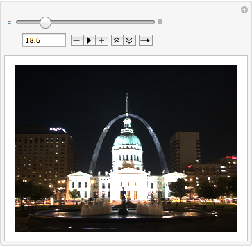
Manipulate[ImageMultiply[hdrimage, \[Alpha]], {{\[Alpha], 1}, 1, 100}]

Also we could now start compressing the dynamic range again by applying tone mapping algorithms and the like.

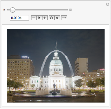
Update An example for an easy global tone mapping algorithm can be achieved by applying #/(#+C) & to every pixel intensity which looks like this:

Manipulate[
  ImageApply[#/(# + \[Alpha]) &, hdrimage], {{\[Alpha], 0.2}, 0.001, 0.2}
]

Answer 3

Version 9 answer - use built-in functionality

The symbols Image`CreateHDRI and Image`ToneMapHDRI were present in version 8 but didn't seem to do anything. In version 9 there is functioning code behind them. This is all undocumented, and therefore liable to change before it is officially released, but here is what I've managed to dig up.

Image`CreateHDRI

This function takes a list of images at different exposures and composes them into a single high dynamic range image. The basic usage is simply

Image`CreateHDRI[{image1, image2, ...}, options]

The following default options are defined:

Options[Image`CreateHDRI]
(* {"ExposureTimes" -> {}, "EV" -> {},
    "GenerateCameraResponseFunction" -> True, "AlignTranslation" -> False} *)

"ExposureTimes" and "EV" allow you to provide a list of known exposure times or exposure values. If both are left at the default empty list setting, the exposure times will be computed from the images.

"AlignTranslation" can be set to True to align the images prior to combining them. As the name suggests, the alignment is translation only, scale and rotation errors are not handled.

"GenerateCameraResponseFunction" presumably generates a camera response function :-) This takes suboptions, which default to {"Variance" -> 16., "PredefinedResponse" -> "Linear"}. Other settings for the predefined response curve are "Log10" and "Gamma". I'm not sure what the "Variance" setting does, or what happens if "GenerateCameraResponseFunction" is set to False.

Image`ToneMapHDRI

This function takes a single HDR image and applies one of a variety of tone-mapping algorithms, which are specified in a Method option. The default is:

Options[Image`ToneMapHDRI]
(* {Method -> "PhotographicToneReproduction"} *)

The available algorithms are:

algos = Image`HDRImageProcessingDump`$ToneMapAlgos
(* {"AdaptiveLog", "Photoreceptor", "FattalGradientDomain", 
     "PhotographicToneReproduction", "ContrastDomain"} *)

Each algorithm has a set of sub-options, the default settings are:

{#, Image`HDRImageProcessingDump`defaultsuboptions[#]}& /@ algos

(* {{"AdaptiveLog", {"Bias" -> 0.8, "Gamma" -> 1., "Saturation" -> 1.}},
 {"Photoreceptor", {"LuminousIntensity" -> 0., "ChromaticAdaptation" -> 0., "LightAdaptation" -> 1., "OverallContrast" -> 0.}},
 {"FattalGradientDomain", {"Threshold" -> 0.1, "Order" -> 0.8, "ParamX" -> Automatic, "Saturation" -> 0.8}},
 {"PhotographicToneReproduction", {"Key" -> 0.18, "Sharpening" -> 8., "UseLocalOperator" -> False, "NumberOfScales" -> 8, "SmallestScale" -> 1, "LargestScale" -> 43, "Saturation" -> 0.8}},
 {"ContrastDomain", {"ContrastScaleFactor" -> 0.3, "UseContrastEqualization" -> True, "Saturation" -> 0.8}}} *)

Not being an expert in HDR tone-mapping algorithms, I can't really comment on what these parameters control, but it is easy enough to play around with the values and see the results.

Example

Here is an example of processing the Stanford Memorial Church images with the new functionality:

(* load the source images *)
files = Reverse@FileNames["memorial*.png"];
images = ImagePad[Import[#], {{-2, -12}, {-35, -30}}] & /@ files;

(* create the HDR image *)
i = Image`CreateHDRI[images];

(* apply a tone-mapping algorithm *)
Image`ToneMapHDRI[i, Method -> {"FattalGradientDomain", {"Threshold" -> 0.3}}]

Answer 4

Exposure fusion is often a powerful alternative to the reconstruction of HDR images if we are only interested in the tone mapped result. HDR reconstructions are often not possible because exposure times are not available or hard to estimate from the given set of images. Many exposure fusion algorithms are also very fast and therefore suitable for real time applications. So I thought it can't hurt to post another such algorithm.

The idea behind the algorithm is to blend the images in a way so that the level of detail in the final image is maximal.

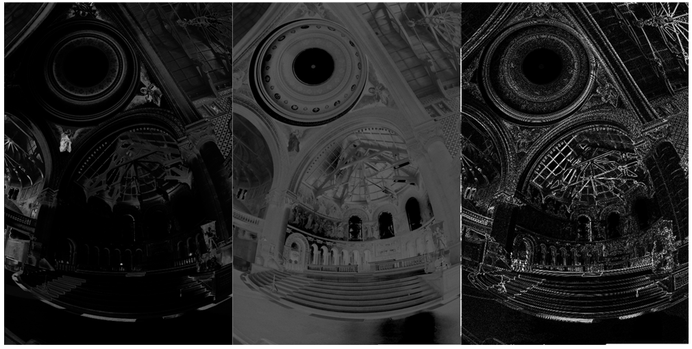
First each image is weighted by three quality measures, well-exposedness, saturation and contrast. The three weight maps are combined and normalised over all images. Three example weights are shown.

images = Image[Import["..\\memorial00" <> ToString@# <> ".png"], "Real"]
    & /@ Range[61, 76];

WellExposedness[img_] := Module[
  {ch = ColorSeparate@img},
  ImageMultiply @@ (ImageApply[Exp[-(# - 0.5)^2/0.08] &, #] & /@ ch)]
SaturationMeasure[img_] := 
 ImageApply[StandardDeviation@# + 10^-10 &, img]
ContrastMeasure[img_] := 
 ImageApply[Abs@# + 10^-10 &, 
  LaplacianFilter[ColorConvert[img, "Grayscale"], 10]]

ImageWeightMap[img_, {a_, b_, c_}] := ImageMultiply @@ {
   ImageApply[#^a &, WellExposedness[img]],
   ImageApply[#^a &, SaturationMeasure[img]],
   ImageApply[#^a &, ContrastMeasure[img]]}

NormalizeWeightmaps[weightmaps_] := Module[
  {weightmapSum = ImageApply[1/# &, ImageAdd @@ weightmaps]},
  ImageMultiply[weightmapSum, #] & /@ weightmaps]

ImageAssemble[{{WellExposedness@images[[1]],
   SaturationMeasure@images[[1]],
   ContrastMeasure@images[[1]]}}]

Simple blending of the images using the generated weight maps can introduce ugly boundaries between the image parts as shown in the following example where only 2 images of the set are blended.

SimpleExposureBlend[images_, {exp_, sat_, con_}] := Module[
  {imgN = Length@images,
   wm = ImageWeightMap[#, {exp, sat, con}] & /@ images,
   wmNorm},
  wmNorm = NormalizeWeightmaps[wm];
  ImageAdd @@ MapThread[ImageMultiply[#1, #2] &, {images, wmNorm}]
  ]

SimpleExposureBlend[images, {1, 1, 1}]

This issue can be avoided by using multi-scale pyramid blending to combine the images.

ImagePyramidDepth = Length[NestWhileList[Ceiling[#/2] &, #, Ceiling[#] != 1 &]] - 1 &;
GaussPyramid[img_, depth_, kernel_: GaussianMatrix[2], re_: "Gaussian"] := 
    Module[{},NestList[ImageResize[ImageConvolve[#, kernel], Scaled[1/2], 
    Resampling -> re] &, img, depth]];
LaplacePyramid[img_, depth_, kernel_: GaussianMatrix[2], re_: "Gaussian"] := 
 Module[{Gpy = GaussPyramid[img, depth, kernel, re]},
    Join[ImageSubtract[#1, 
      ImageResize[#2, Scaled[2], Resampling -> re]] & @@@ 
    Partition[Gpy, 2, 1], {Last@Gpy}]]
CollapseLaplacePyramid[lapPyr_, re_: "Gaussian"] :=
    ImageAdjust@Fold[ImageAdd[#1, 
    ImageResize[#2, ImageDimensions@#1, Resampling -> re]] &, 
    First@lapPyr, Rest@lapPyr]

MultiLevelExposureBlend[images_, {exp_, sat_, con_}] := Module[
  {imgN = Length@images,
   wm = ImageWeightMap[#, {exp, sat, con}] & /@ images,
   pyrDepth = ImagePyramidDepth@Min@ImageDimensions@images[[1]],
   wmNorm, gp, lp, blend},
  wmNorm = NormalizeWeightmaps[wm];

  gp = GaussPyramid[#, pyrDepth] & /@ wmNorm;
  lp = LaplacePyramid[#, pyrDepth] & /@ images;
  blend = ImageAdd @@ # & /@ Transpose[
     ImageMultiply @@@ # & /@ (Transpose[{#1, #2}] & @@@ Transpose[{gp, lp}])];
  CollapseLaplacePyramid@blend
  ]

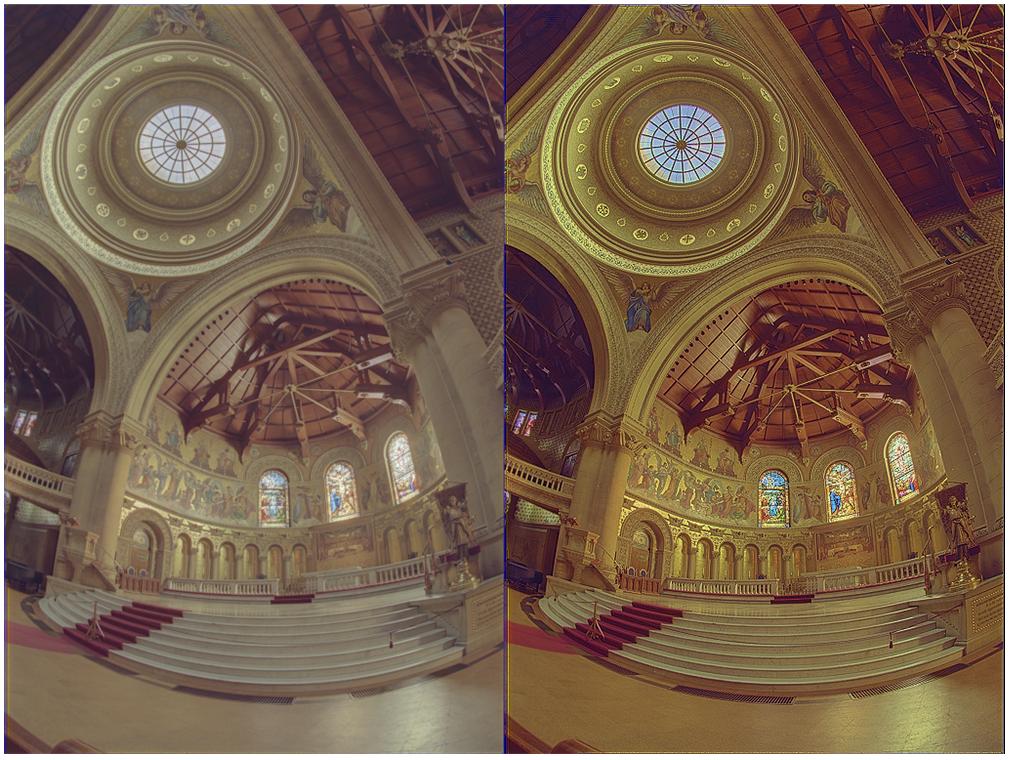
i1 = MultiLevelExposureBlend[images, {1, 1, 1}];
i2 = ImageAdjust[ColorCombine[{#1, ImageAdjust[#2, {0, 0, 0.5}],
       Nest[Sharpen[#, 1] &, #3, 3]} & @@ ColorSeparate[ColorConvert[i1, "HSB"]], "HSB"]];
ImageAssemble[{i1, i2}]

relevant paper