Fixing phase unwrapping jumps

Question

The problem of unwrapping 1D phase often comes up in Fourier analysis: someone computes a DFT of some data, the resulting phase values fall between $-\pi$ and $\pi$, and they'd like to "unwrap" these phase values to not be bounded to (-$\pi$,$\pi$]. It's fairly straightforward in the case of low noise and sufficient discrete sampling, as seen in the excellent answers here.

However, by working more with the continuous case and/or no noise, the essential problems typically associated with 1D phase unwrapping are not dealt with. Here's an example of where things can go wrong in a discrete case with some noise and limited sampling.

phaseUnwrap[vec_?VectorQ] := (*translation of Matlab's implementation*)
 Module[{n = Length[vec], ph = Arg[vec], df}, 
  df = Differences[ph]; 
  Do[ph -=
2 Pi Sign[df[[k]]] PadRight[ConstantArray[0, k], n, 1],
 {k, Flatten[
 Position[
  Abs[df], _?(# > Pi &)]]}]; ph];

data = Import["http://pastebin.com/raw/haAxt0br", "Package"];

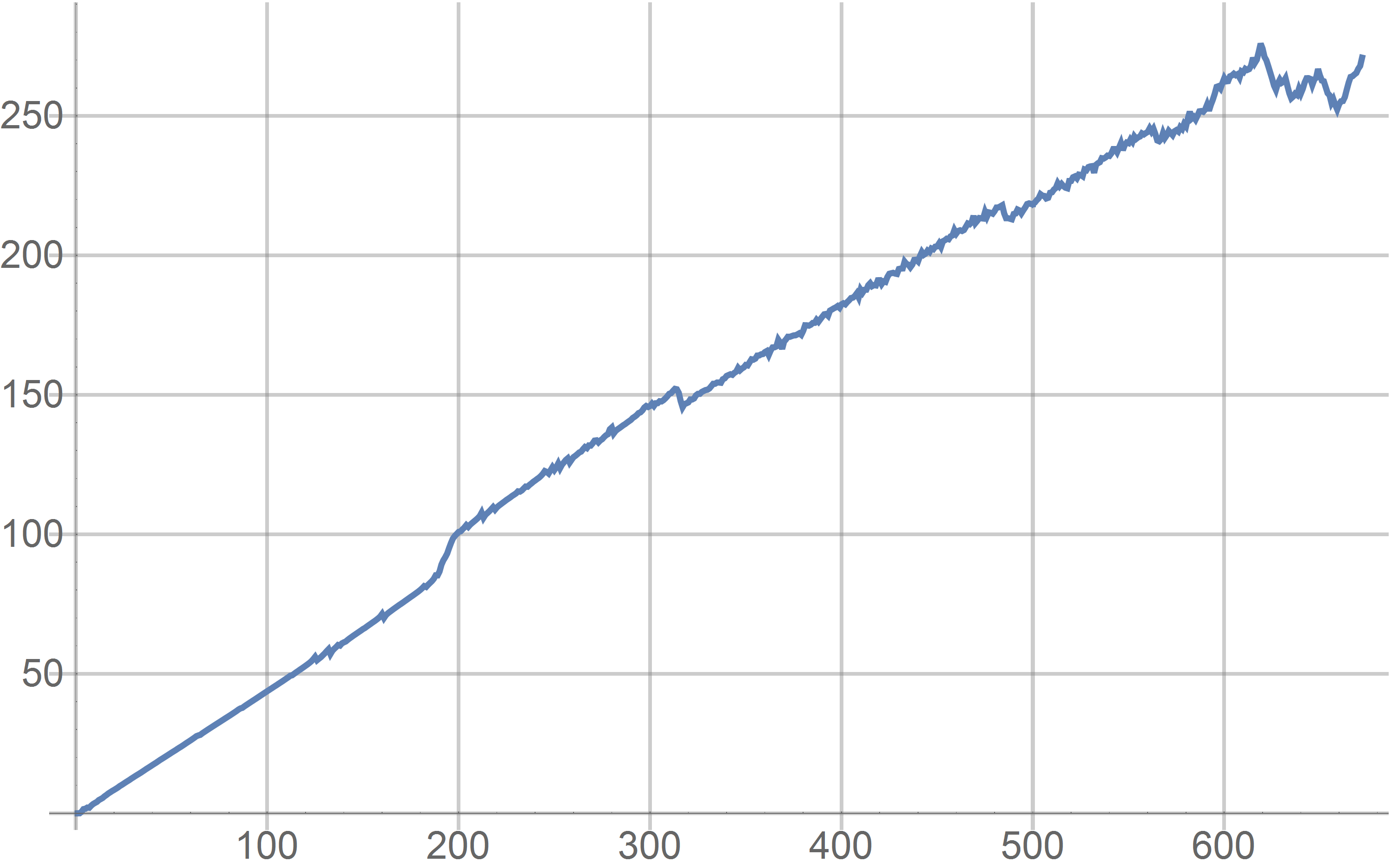
ListPlot[phaseUnwrap[data[[;; , 2]]], Joined -> True]

Even with noise and low-ish sampling the algorithm does a pretty good job, but there are still some obvious jumps in the phase unwrapping process, notably just after point 300 and just before point 500.

Given how easy it is to pick these out by eye, it seems like there could be a simple way to correct them. Maybe minimizing the derivative somehow? Checking afterward for deviations from a linear fit?

Answer 1

Alright, I found a decent way to do this given some assumptions about what the shape of the data "should" be. This is a post-processing function, i.e., it should be applied after a function like phaseUnwrap. Essentially I assume that the data should be linear, and further that in some part of the domain there is already a nice linear region. As input we take the lower and upper bounds of this region, as well as the messy unwrapped data.

magnetize[phaseData_, lower_, upper_] :=
 Module[{fitdata, fit, magnet, magnetizedData, tries},
  fitdata = Transpose[{
 Range[lower, upper],
 phaseData[[lower ;; upper]]}];
 fit = LinearModelFit[fitdata, x, x];
 magnet = First@Last@Reap@
      For[i = 1, i < (Length@phaseData + 1), i++,
   tries = Sort[
     Table[{k, 
       Abs[(fit[i] - phaseData[[i]] - (2 Pi k))]}, {k, -10, 10, 1}],
     #1[[2]] > #2[[2]] &];
   Sow[
    tries[[-1, 1]]]];
  magnetizedData = phaseData + 2 Pi magnet;
  {magnetizedData, fit,
 Show[{ListPlot[{phaseData, magnetizedData}, Joined -> True, 
  GridLines -> {Automatic, Automatic},
  Epilog -> {
    Line[{{lower, 0}, {lower, 300}}],
    Line[{{upper, 0}, {upper, 300}}]}],
 Plot[fit[x], {x, 0, Ceiling@(1.1*Length@phaseData)},
  PlotStyle -> Directive[Gray]]
 }]}
]

In summary,

1. Find a linear fit line based on a "nice" part of the data
2. For every point, find the integer multiple of $2\pi$ that brings the data closest to the fit line.
3. Return {processed data, fit line object, plot}

It's a little rough but it gets the job done.

mag1 = magnetize[phaseUnwrap[data[[;; , 2]]], 50, 120];   
(*using data and function from the question post *) 
mag1[[3]]