3
$\begingroup$

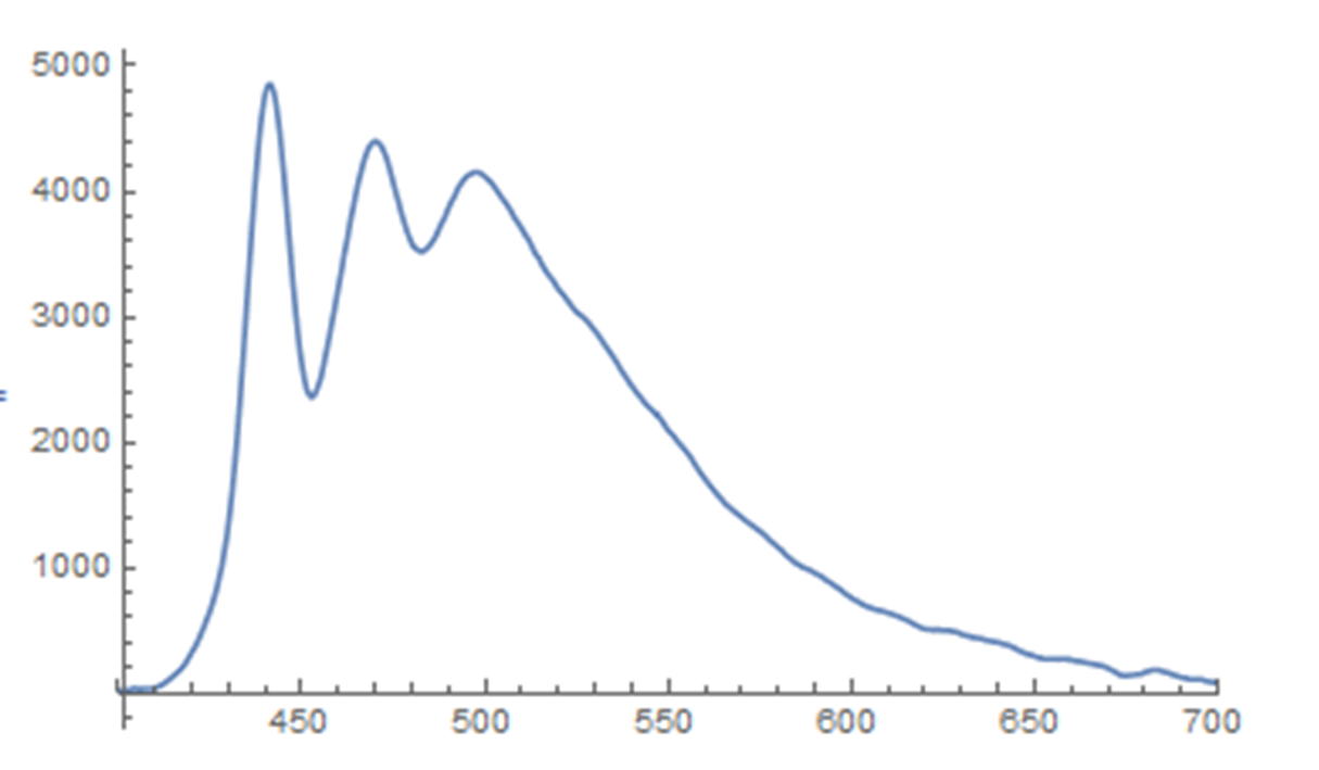
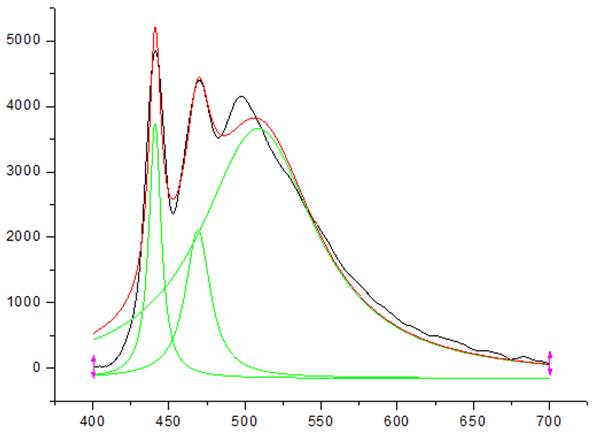
For example, I have the next spectrum:

enter image description here

I've seen the next question ["How to perform a multi-peak fitting?"][2]

but not answer to my question. I want deconvolution the spectrum to obtain three peaks (how Origin to do it). The sum of these three peaks gives the total spectrum. I know fit each peaks with gaussian or lorentziana function (or mixture of both) but this is different to deconvolution. My interest for deconvolution is find the FWHM each peak.

Are there codes for deconvolution data similar to mine?.

These are the datas of the spectrum: Spectrum data

[2]: How to perform a multi-peak fitting? multi-peak-fitting This the code with the function for fitting each peak:

modelL = (2*A/Pi)*(w/(4*(x - xc)^2 + w^2));
modelGfh = A/(w*Sqrt[Pi/4 Log[2]])*E^(-4*Log[2]*(x - xc)^2/w^2);
r = 0.2;
modelLGfh = r*modelL + (1 - r)*modelGfh;
nlmD = NonlinearModelFit[peak1, 
modelLGfh, {{A, 1}, {w, 1}, {xc, 441}}, x, MaxIterations -> 10000];
$\endgroup$
5
  • $\begingroup$ What function are the peaks convolved with? $\endgroup$ Commented Sep 6, 2016 at 16:13
  • $\begingroup$ The spectrum is a list {x,y} of datas. $\endgroup$
    – Manu
    Commented Sep 6, 2016 at 16:20
  • $\begingroup$ It seems to me that what you are asking can be answered by (1) finding local maximums and (2) using NonlinearModelFit for Gaussian functions that have those local maximums as peaks. $\endgroup$ Commented Sep 6, 2016 at 16:32
  • $\begingroup$ Is there actual data for this example? $\endgroup$ Commented Sep 6, 2016 at 16:48
  • $\begingroup$ @Manu Please see my preliminary answer. If it is close to what you want I can improve with more details and better fitting results. $\endgroup$ Commented Sep 6, 2016 at 17:10

3 Answers 3

6
$\begingroup$

Not a complete answer. I want to hear from OP is this what he wants, then I can provide a full answer.

Getting data

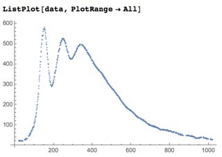
It would be good if data for the plot is provided in question. I extracted data points from the image attached to the question using the process described in the discussion "Recovering data points from an image".

enter image description here

Finding local extrema

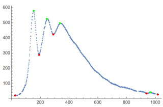
Using this answer I found the local extrema.

enter image description here

Here are the peaks:

In[136]:= peaks = extrema[[2, 1 ;; 3]] 
Out[136]= {{153, 580.}, {245, 527.}, {335, 498.}}

Non-linear model fitting

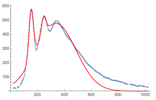
For the three peaks we can generate three Gaussian functions and use Non-linear model fitting for their weighted sum.

Here are the functions:

In[196]:= fitFuncs = 
 Table[a[i] peaks[[i, 2]] PDF[NormalDistribution[peaks[[i, 1]], s[i]],
     x], {i, 3}]

Out[196]= {(231.387 E^(-((-153 + x)^2/(2 s[1]^2))) a[1])/s[1], (
 210.243 E^(-((-245 + x)^2/(2 s[2]^2))) a[2])/s[2], (
 198.673 E^(-((-335 + x)^2/(2 s[3]^2))) a[3])/s[3]}

Here is the fitting (with constraints):

nlm = NonlinearModelFit[
  data, {Total[fitFuncs], {0 < a[1], 0 < a[2], 0 < a[3], 
    0 < s[1] < 20, 0 < s[2] < 30, 0 < s[3] < 150}}, 
  Join[Array[a, 3], Array[s, 3]], x]

Here are the found parameters:

In[226]:= nlm["BestFitParameters"]   
Out[226]= {a[1] -> 24.9994, a[2] -> 10.4565, a[3] -> 362.068, 
 s[1] -> 16.5082, s[2] -> 16.9777, s[3] -> 150.}

Plotting data and the fitted function:

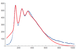
enter image description here

Quantile regression

Similar fitting for another MSE question, "Fit a function to data so that fit is always equal or less than the data", makes me think that with Quantile Regression we can get better results.

In[23]:= qfunc

Out[23]= 0. + 7.92161 E^(-0.005 (-335 + x)^2) + 
 50.8584 E^(-0.00125 (-335 + x)^2) + 
 53.4119 E^(-0.00005 (-335 + x)^2) + 
 381.914 E^(-0.0000125 (-335 + x)^2) + 
 9.10845 E^(-0.00138504 (-245 + x)^2) + 
 136.737 E^(-0.00131492 (-245 + x)^2) + 
 167.451 E^(-0.00274348 (-153 + x)^2) + 
 145.583 E^(-0.00255102 (-153 + x)^2)

In[22]:= Show[ListPlot[data, PlotRange -> All],
 Plot[qfunc, {x, Min[data[[All, 1]]], Max[data[[All, 1]]]}, 
  PlotStyle -> Red, PlotRange -> All]]

enter image description here

$\endgroup$
4
  • $\begingroup$ thank so much for your help. I've the similar result to your answer. My interest to deconvolution is find the FWHM each peak. I fitting each peak with a Gaussian plus Lorentziana function and then I can obtain the FWHM. I obtain this: !Spectrum $\endgroup$
    – Manu
    Commented Sep 6, 2016 at 18:17
  • $\begingroup$ @Manu Please list or specify with concrete formulas in your question what functions you want to fit. Also provide data. $\endgroup$ Commented Sep 6, 2016 at 18:23
  • $\begingroup$ Howerer, this is an approximation. For find the real FWHM of each peak is necessary deconvolution the spectrum. $\endgroup$
    – Manu
    Commented Sep 6, 2016 at 18:26
  • $\begingroup$ I've edited the question. I provide the data and the function that I use for fit each peak. $\endgroup$
    – Manu
    Commented Sep 6, 2016 at 18:40
7
$\begingroup$

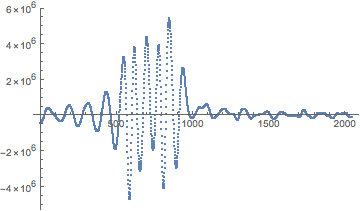
I don't think deconvolution is what you are really after. For example, there is a function called ListDeconvolve. Let's apply it to your data. First you need to specify a kernel for the deconvolution. Let's try a kernel that's a Gaussian of width 50:

gauss = GaussianMatrix[100][[50]];
ListPlot[ListDeconvolve[gauss, data], PlotRange -> All]

enter image description here

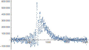
Now try a kernel of length 15:

gauss = GaussianMatrix[30][[15]];
ListPlot[ListDeconvolve[gauss, data2], PlotRange -> All]

enter image description here

Neither is very satisfying because your peaks are of different widths. Deconvolution will only work if all three peaks are of roughly the same width (since you deconvolve the same kernel across the whole data set). So I think you are going to need to do something more like peak-picking as suggested by Anton.

$\endgroup$
1
  • $\begingroup$ Nice clarification. (+1) $\endgroup$ Commented Sep 6, 2016 at 19:20
1
$\begingroup$

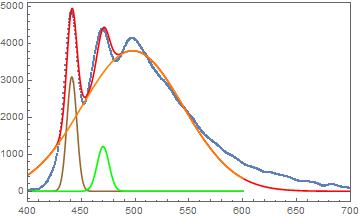
I've analized the Anton Antonov solution with Non-linear model fitting:

peaks = Pick[sp[[630 ;; 880]], 
PeakDetect[sp[[630 ;; 880]][[All, 2]], 3.6, 0.05], 1]

fitFuncs = 
Table[a[i] peaks[[i, 2]] PDF[
NormalDistribution[peaks[[i, 1]], s[i]], x], {i, 3}];

nlm = NonlinearModelFit[
sp, {Total[fitFuncs], {0 < a[1], 0 < a[2], 0 < a[3], 0 < s[1] < 20,
0 < s[2] < 30, 0 < s[3] < 150}}, Join[Array[a, 3], Array[s, 3]],
x];

nlm["BestFitParameters"];

a[1] = 7.377124955087864`; s[1] = 4.600197878756341`;
f1[x_] := fitFuncs[[1]];

a[2] = 3.840415143057309`; s[2] = 5.554311215744846`;
f2[x_] := fitFuncs[[2]];

a[3] = 107.9493889229601`; s[3] = 46.89436652386362`;
f3[x_] := fitFuncs[[3]];

Show[ListPlot[sp, PlotRange -> {{400, 700}, All}, Frame -> True, 
FrameTicks -> {{Automatic, None}, {Automatic, None}}], 
Plot[nlm[x], {x, 400, 700}, PlotRange -> All, PlotStyle -> Red, 
Frame -> True, 
FrameTicks -> {{Automatic, None}, {Automatic, None}}], 
Plot[f1[x], {x, 400, 600}, PlotStyle -> Brown, PlotRange -> All, 
Frame -> True, 
FrameTicks -> {{Automatic, None}, {Automatic, None}}], 
Plot[f2[x], {x, 400, 600}, PlotStyle -> Green, PlotRange -> All, 
Frame -> True, 
FrameTicks -> {{Automatic, None}, {Automatic, None}}], 
Plot[f3[x], {x, 400, 600}, PlotStyle -> Orange, PlotRange -> All, 
Frame -> True, 
FrameTicks -> {{Automatic, None}, {Automatic, None}}]]

enter image description here

This results is very aproximated to deconvolution in Origin for example:

enter image description here

The results will improve using the Lorentziana plus Gaussiana function and/or Quantile regression that Anton Antonov indicated in his answer. just change the functions in the fitFuncs line.

$\endgroup$

Your Answer

By clicking “Post Your Answer”, you agree to our terms of service and acknowledge you have read our privacy policy.

Not the answer you're looking for? Browse other questions tagged or ask your own question.