Sebastian mentioned in his answer that deepdream can be possible using NetDerivative. Here are my attempts following his outlines.
Instead of using the inception model, I'm using VGG-16 here for simplicity. Inception model allows arbitrary image size, but may need some extra normalization steps.
The MXNet version of the VGG model can be downloaded from MXnet's github page https://github.com/dmlc/mxnet-model-gallery
The VGG model can be loaded as
Needs["NeuralNetworks`"]
VGG = ImportMXNetModel["vgg16-symbol.json", "vgg16-0000.params"]

The VGG is trained by 224 by 224 images, so we will load and crop our test image to this size
img = RemoveAlphaChannel@
  ImageCrop[
   Import["http://hplussummit.com/images/wolfram.jpg"], {224, 224},
   Padding -> None]

We can then take the network up to the layer at which we want maximum activation, and then attach a SummationLayer
net = NetChain[{Take[VGG, {"conv1_1", "pool1"}], SummationLayer[]},
  "Input" -> NetEncoder[{"Image", {224, 224}}]]
We then want to back propagate to the input, and find the gradient this respect to the value at the summation layer. This can be done with NetDerivative. This is what the gradient looks like
NetDecoder["Image"][
 First[(NetDerivative[net]@<|"Input" -> img|>)[
   NetPort["Inputs", "Input"]]]]
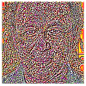
We can now add the gradient to the input image, and calculate the gradient with respect this new image, and so and so forth. This process can also be understood as gradient ascent. Here is the function that does one step of gradient ascent
applyGradient[net_, img_, stepsize_] :=
 Module[{imgt, gdimg, gddata, max, dim},
  gdimg =
   NetDecoder["Image"][
    First[(NetDerivative[net]@<|"Input" -> img|>)[
      NetPort["Inputs", "Input"]]]];
  gddata = ImageData[gdimg];
  max = Max@Abs@gddata;
  Image[ImageData[img] + stepsize*gddata/max]
  ]
We can then apply this repeatedly to our input image and get a deepdream like image
Nest[applyGradient[net, #, 0.1] &, img, 10]
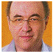
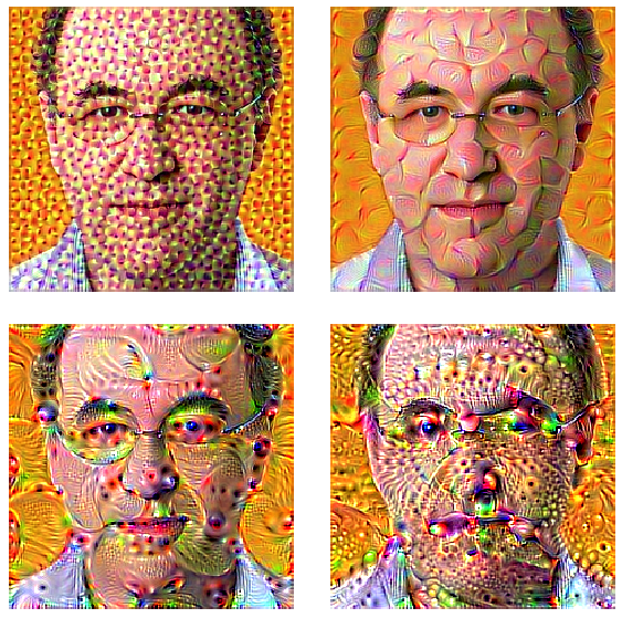
Here are the dreamed image at different pooling layers. When we dream at early pooling layer, localized simple features show up. And as we get to later layers of the network, more complexity features emerges.
dream[img_, layer_, stepsize_, steps_] := Module[{net},
  net = NetChain[{Take[VGG, {"conv1_1", layer}], SummationLayer[]},
    "Input" -> NetEncoder[{"Image", {224, 224}}]];
  Nest[applyGradient[net, #, stepsize] &, img, steps]
  ]

Show[ImagePad[dream[img, #1, #2, #3], 10, White],
    ImageSize -> {224, 224}] & @@@ {{"pool2", 0.1, 10}, {"pool3", 0.1,
     10}, {"pool4", 0.2, 20}, {"pool5", 0.5, 20}} // Row
The way to generate the deep-dream images can also be used to visualize the convolution layers in the model. To visualize on convolution kernel, we can attach a fully connected layer right after the convolution layer that keeps only one of the filter channel and zero all others.
weights[n_] := List@PadRight[Table[0., n - 1]~Join~{1.}, 1000]
maxAtLayer[img_, n_] := Module[{net, result},
  net = NetChain[{Take[VGG, {"conv1_1", "conv5_3"}], FlattenLayer[],
     DotPlusLayer[1, "Weights" -> weights[n], "Biases" -> {0}],
     SummationLayer[]},
    "Input" -> NetEncoder[{"Image", {224, 224}}]];
  Nest[applyGradient[net, #, 0.01] &, img, 30];
  result
  ]

img = Image[(20*RandomReal[{0, 1}, {224, 224, 3}] + 128)/255.];

maxAtLayer[img, RandomInteger[{1,512}]]

The same can be applied to the last layer of the network
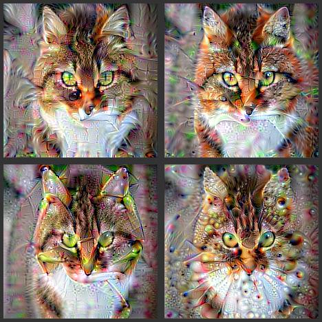

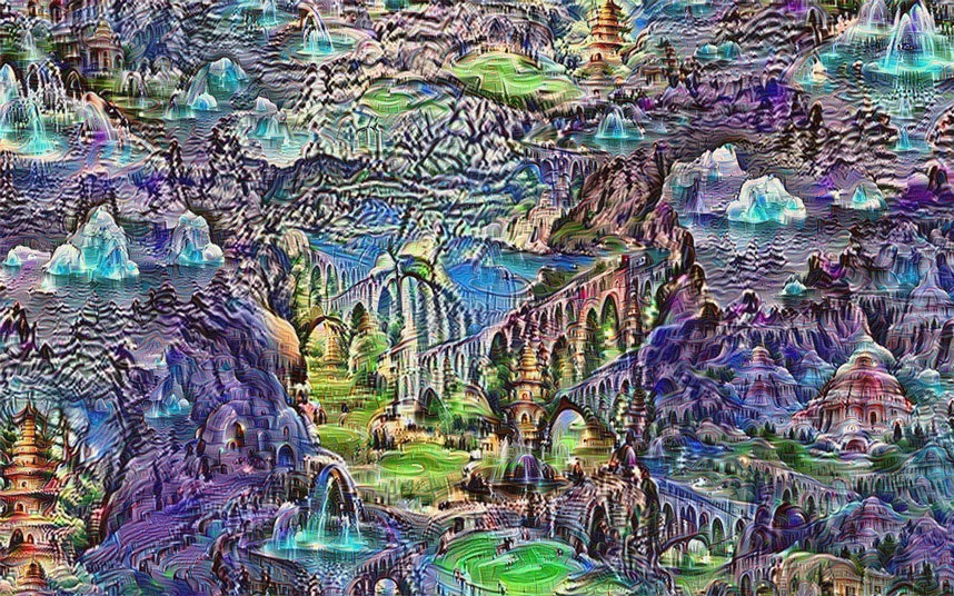
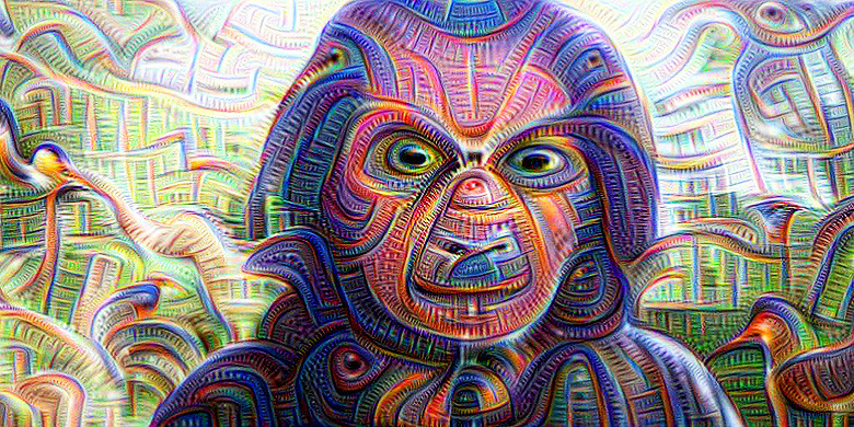


ImageIdentify, but he didn't talk about how he made it. $\endgroup$