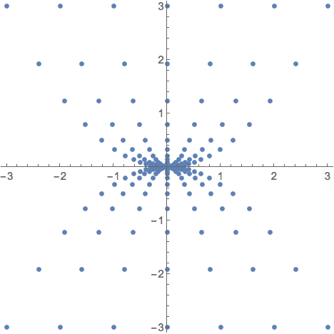
The following image contains solution trajectories of the system:
$$\vec x_{k+1}= \begin{bmatrix} 0.80 & 0\\ 0 & 0.64 \end{bmatrix}\,\vec x_k $$ I've managed to do this:
Clear[A, pts1, pts2, pts]
A = {{.80, 0}, {0, .64}};
pts1 = Table[NestList[A.# &, {k, 3}, 20], {k, -3, 3}];
pts2 = Table[NestList[A.# &, {k, -3}, 20], {k, -3, 3}];
pts = Flatten[Join[pts1, pts2], 1];
ListPlot[pts,
 PlotStyle -> PointSize[Medium],
 PlotRange -> {{-3.1, 3.1}, {-3.1, 3.1}},
 AspectRatio -> Automatic]
Which gives this image:
What I would like to learn how to do is to include a smooth curve for each trajectory, points of the trajectory lying on the curve, and a little arrow on each curve pointing in the direction of the origin.
I'd appreciate any help.
Thanks.
Update: Thanks to some nice help from cyrille.piatecki and Sumit, I was able to produce this:
Clear[A, pts1, pts2, pts]
A = {{.80, 0}, {0, .64}};
pts1 = Table[NestList[A.# &, {k, 3}, 10], {k, -3, 3}];
pts2 = Table[NestList[A.# &, {k, -3}, 10], {k, -3, 3}];
pts = Join[pts1, pts2];
Show[
 ListLinePlot[pts,
   InterpolationOrder -> 2,
   AxesLabel -> {"\!\(\*SubscriptBox[\(x\), \(1\)]\)",
     "\!\(\*SubscriptBox[\(x\), \(2\)]\)"},
   PlotRange -> {{-3.3, 3.3}, {-3.1, 3.1}},
   AspectRatio -> Automatic,
   Epilog -> {
     Text[
      Style["\!\(\*SubscriptBox[\(x\), \(0\)]\)", 12, Black], {3,
       3}, {-1, 1}],
     Text[
      Style["\!\(\*SubscriptBox[\(x\), \(1\)]\)", 12, Black], {2.4,
       1.92}, {-1, 1}],
     Text[
      Style["\!\(\*SubscriptBox[\(x\), \(2\)]\)", 12, Black], {1.92,
       1.23}, {-1, 1}],
     Text[
      Style["\!\(\*SubscriptBox[\(x\), \(0\)]\)", 12, Black], {-3,
       3}, {1, 1}],
     Text[
      Style["\!\(\*SubscriptBox[\(x\), \(1\)]\)", 12, Black], {-2.4,
       1.92}, {1, 1}],
     Text[
      Style["\!\(\*SubscriptBox[\(x\), \(2\)]\)", 12, Black], {-1.92,
       1.23}, {1, 1}]
     }] /. Line[x_] -> {Arrowheads[{0., 0.04, 0.}], Arrow[x]},
 ListPlot[pts,
  PlotStyle -> PointSize[0.015]]
 ]
Which produced this image:


