Constructing a root solution diagram (not to tell bifurcation)

Question

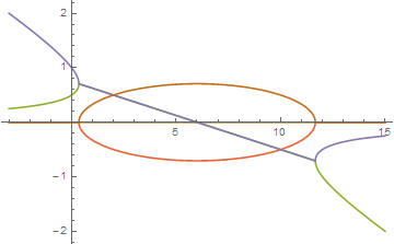
Suppose I have a third order equation depending of one parameter say

.5 4 x (1 - x) (x - .5) - .5 m x^2

where m the parameter. Obviously there are 3 roots for each value of m but two of them may be multiple or Complex

I want to construct a graphic $(t, x^\star)$ showing for wich subset of $\mathbb{R}$ there is 3, 2 or 1 real root(s) ---and of course to plot it. I have tried many way to program this functionaly. The problem is that in presence of multiple roots Mathematica shows only two roots. For instance

l = Range[0, 2, .01];
Length[l]
SetAttribute[f, Listable]
f[m_] := Solve[.5 4 x (1 - x) (x - .5) - .5 m x^2 == 0, x]

If I print

 zT := Table[{l[[i]], f[i]}, {i, 1, 80}]

I can observe that the first term $\{0., \{\{x -> 0.\}, \{x -> 1.\}\}\}$ of zT returns only two values. So there is not third term as for all the other elements of zT. I know that I will be obliged to refer to the absence of the third term.

I have tried to construct Three lists as follow :

zOn := Table[{l[[i]], If[Im[f[i][[1, 1, 2]]] != 0, 0, f[i][[1, 1, 2]]]}, {i, 1, 80}]
zTw := Table[{l[[i]], If[Im[f[i][[2, 1, 2]]] != 0, 0, f[i][[2, 1, 2]]]}, {i, 1, 80}]

zTh := Table[{l[[i]], If[Im[f[i][[3, 1, 2]]] != 0, 0, f[i][[3, 1, 2]]]}, {i, 1, 80}]

because 0 is always an equilibrium. I have planned to ListLinePlot them. But unfortunately, my approach fails because the first term is compose only of two rules. I have thought to construct a second condition which would state that there doesn't exist a third term like If Im[f[i][[2, 1, 2]]] != 0 Or (A 3 term does not exist) but I don't know how to do that --- How to program the rule If part[3] of f[i] does not exist

The question is important for research reason but also because I try to forget procedural programming and use only fonctional programming.

Answer 1

Maybe you want something like this?:

eq = 4/2 x (1 - x) (x - 1/2) - 1/2 m x^2

sols = x /. Solve[expr == 0, x]
(* Out[2] := {0,1/8 (6-m-Sqrt[4-12 m+m^2]),1/8 (6-m+Sqrt[4-12 m+m^2])} *)

realandimaginarysolutions = Through[{Re, Im}[#]] & /@ sols
(* Out[3] := {{0,0}
             ,{1/8 (6+Re[-m-Sqrt[4-12 m+m^2]]),1/8 Im[-m-Sqrt[4-12 m+m^2]]}
             ,{1/8 (6+Re[-m+Sqrt[4-12 m+m^2]]),1/8 Im[-m+Sqrt[4-12 m+m^2]]}} *)

Plot[realandimaginarysolutions, {m, -3, 15}]

Here we generate the parametrized general (complex valued) solutions first, and extract their real and imaginary part (which are all real valued) and plot those as functions of m.