How do I get rid of a "jump" in my plot?

Question

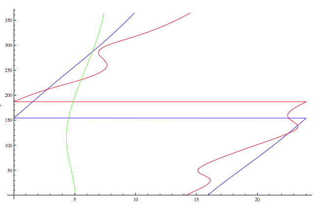
How can I prevent plotting functions from "connecting" inside a plot points that should "wrap around" outside the plot?

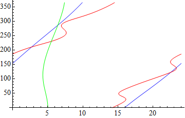
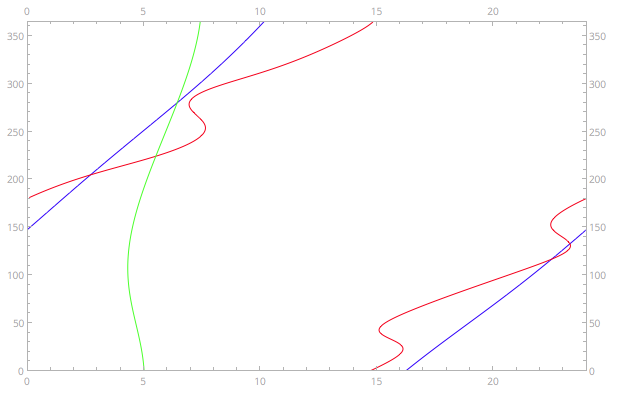
For example, how do I eliminate the horizontal lines running across the following ParametricPlot?

enter image description here

In this figure, the paths that reach the right hand end of the graph at 24 should continue at 0 (these are hours, so 24=0) without passing backwards across the figure.

Show[
 ParametricPlot[
  {AstronomicalData[
    "Mars", {"RightAscension", 
     DatePlus[Date[], d], {$GeoLocation[[1]] , $GeoLocation[[2]]}}], d},
  {d, 0, 365}, AspectRatio -> 1/1.6, PlotStyle -> Blue],
 ParametricPlot[
  {AstronomicalData[
    "Mercury", {"RightAscension", 
     DatePlus[Date[], d], {$GeoLocation[[1]] , $GeoLocation[[2]]}}], d},
  {d, 0, 365}, AspectRatio -> 1/1.6, PlotStyle -> Red],
 ParametricPlot[
  {AstronomicalData[
    "Jupiter", {"RightAscension", 
     DatePlus[Date[], d], {$GeoLocation[[1]] , $GeoLocation[[2]]}}], d},
  {d, 0, 365}, AspectRatio -> 1/1.6, PlotStyle -> Green]
 ]

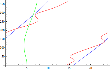
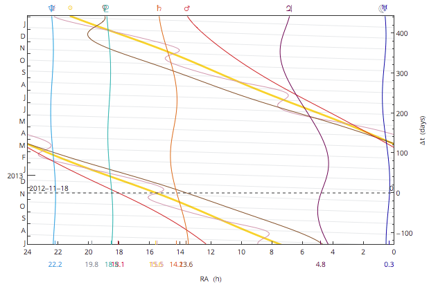
FWIW, the (almost) final result, with help from SE: enter image description here

Note, this code is absurdly slow, but that's another question. — orome, Commented Oct 8, 2012 at 3:43
Can't investigate at the moment (I suspect this is a matter of inverse trig branch cuts, though; see this), but: you can replace {$GeoLocation[[1]] , $GeoLocation[[2]]} with Take[$GeoLocation, 2]. — J. M.'s missing motivation, Commented Oct 8, 2012 at 4:17
@J.M.: Good point. The code is adapted from cases where the latitude and longitude may be independently replaced, which is why that part is verbose. — orome, Commented Oct 10, 2012 at 14:08

Mr.Wizard · Accepted Answer · 2012-10-08 23:46:29Z

6

Theoretically the Exclusions option should be able to handle this but I couldn't find the right arguments. Therefore I recommend a method similar to Simon's, but I would instead Split the lines where there are any large discontinuities in x :

(* Simon's code *)
plot = Show[MapThread[ParametricPlot[
 {AstronomicalData[#1, {"RightAscension", DatePlus[Date[], d], $GeoLocation}], d},
 {d, 0, 365}, AspectRatio -> 1/1.6, PlotStyle -> #2] &, 
 {{"Mars", "Mercury", "Jupiter"}, {Blue, Red, Green}}]];


plot /. Line[x_] :> Line@Split[x, Norm[# - #2] < 10 &]

Mathematica graphics

answered Oct 8, 2012 at 23:46

Mr.Wizard

273k34 gold badges595 silver badges1.4k bronze badges

$\begingroup$ That certainly looks tidier than my CW answer. But I'm a bit foggy on what's going on with Line and :>. Is there a reason to prefer that approach over simply including the Split in the plot, as in the CW answer? $\endgroup$
– orome
Commented Oct 8, 2012 at 23:52
$\begingroup$ Ah, I think I see the answer. My approach only works because I've "switched" to ListPlot, while this one works for any plot since it's operating on the Line primitive. (And yes, I tired Exclusions but could not get it to work.) $\endgroup$
– orome
Commented Oct 8, 2012 at 23:55
1

$\begingroup$ @rax If you are not familiar with transformation rules you will need to start here. Specifically here the output of ParametricPlot is a Graphics object constructed of primitives such as Line and Options such as PlotRange. My transformation rule (applied with /.) is RuleDelayed (:>) so that the right-hand-side does not evaluate until x is substituted in. Norm is just a short-hand to check the distance between points; EuclideanDistance would work too, perhaps better. $\endgroup$
– Mr.Wizard
Commented Oct 9, 2012 at 0:12
1

$\begingroup$ I used to use this precise strategy of Split[]-ting Line[] objects produced by plotting functions, for removing "long" or "steep" lines in plots, before the Exclusions option came along. I don't know about the advantages of rewriting the splitting test in terms of EuclideanDistance[], but Norm[# - #2] < 10 & is the same as EuclideanDistance[#, #2] < 10 &. $\endgroup$
– J. M.'s missing motivation ♦
Commented Oct 9, 2012 at 7:42
1

$\begingroup$ Ah, Split, much neater! I completely forgot about the existence of Split, even whilst thinking "I need to SPLIT this line into two"... $\endgroup$
– Simon Woods
Commented Oct 9, 2012 at 9:14

| Show 4 more comments

Simon Woods · Accepted Answer · 2012-10-08 19:30:04Z

4

A simple hack for this specific problem is to split each Line primitive into two at the first occurrence of a small x value:

plot = Show[MapThread[ParametricPlot[
 {AstronomicalData[#1, {"RightAscension", DatePlus[Date[], d], $GeoLocation}], d},
 {d, 0, 365}, AspectRatio -> 1/1.6, PlotStyle -> #2] &, 
 {{"Mars", "Mercury", "Jupiter"}, {Blue, Red, Green}}]];

plot /. Line[{pts1__, {x_ /; x < 1, _}, pts2__}] :> {Line[{pts1}], Line[{pts2}]}

enter image description here

answered Oct 8, 2012 at 19:30

Simon Woods

85.4k8 gold badges180 silver badges326 bronze badges

Add a comment |

fizzics · Accepted Answer · 2012-10-08 08:57:22Z

This might be more simplistic than you were looking for but you could always just break it up into several sections and show them together

p1 = ParametricPlot[{AstronomicalData[
"Mars", {"RightAscension", 
 DatePlus[Date[], d], {$GeoLocation[[1]], $GeoLocation[[2]]}}], 
d}, {d, 155, 365}, AspectRatio -> 1/1.6, PlotStyle -> Blue, 
PlotRange -> All, AxesOrigin -> {0, 0}];

p2 = ParametricPlot[{AstronomicalData[
"Mars", {"RightAscension", 
 DatePlus[Date[], d], {$GeoLocation[[1]], $GeoLocation[[2]]}}], 
d}, {d, 0, 154}, AspectRatio -> 1/1.6, PlotStyle -> Blue, 
PlotRange -> All];

p3 = ParametricPlot[{AstronomicalData[
"Mercury", {"RightAscension", 
 DatePlus[Date[], d], {$GeoLocation[[1]], $GeoLocation[[2]]}}], 
d}, {d, 0, 186}, AspectRatio -> 1/1.6, PlotStyle -> Red];

p4 = ParametricPlot[{AstronomicalData[
"Mercury", {"RightAscension", 
 DatePlus[Date[], d], {$GeoLocation[[1]], $GeoLocation[[2]]}}], 
d}, {d, 187, 365}, AspectRatio -> 1/1.6, PlotStyle -> Red];

p5 = ParametricPlot[{AstronomicalData[
"Jupiter", {"RightAscension", 
 DatePlus[Date[], d], {$GeoLocation[[1]], $GeoLocation[[2]]}}], 
d}, {d, 0, 365}, AspectRatio -> 1/1.6, PlotStyle -> Green];

Show[p1, p2, p3, p4, p5]

enter image description here

Then you've changed the problem to writing a piece of code which detects the discontinuities and changes the indices in the plots accordingly. I don't have a chance to do that at the moment but something which measures the distance between successive x-co-ords which stops once the difference is more than a certain threshold you set would get the job done. Mightn't be efficient or tidy but you could generate your plots in an automatic way at least.

detecting the discontinuities could be done with something like this: mf[d_?NumericQ]:=AstronomicalData["Mars",{"RightAscension",DatePlus[Date[],d],{$GeoLocation[[1]],$GeoLocation[[2]]}}]; NMinimize[mf[d], {d, 150, 160}] — sebhofer, Commented Oct 8, 2012 at 9:47
Or even FindMinimum[Abs@mf[d], {d, 155}], which is faster, but less robust and more dependent on well chosen initial conditions. — sebhofer, Commented Oct 8, 2012 at 9:52
This won't help unless in includes a way to locate the spots that need to be excluded. For example, I'd like to put this into a Manipulate were I can change things like the date range dynamically. — orome, Commented Oct 8, 2012 at 13:30
@raxacoricofallapatorius I suggested a way to do this! It might not be the most convenient and robust method though... — sebhofer, Commented Oct 8, 2012 at 14:14

kglr · Accepted Answer · 2012-10-08 13:35:10Z

Using ListLinePlot with Mesh, MeshFunctions, MeshFunctions and MeshShading options. The idea is to change the color of portions to be excluded to White.

First, the data:

 {dataMars, dataMercury, dataJupiter} = 
   Table[{AstronomicalData[#, {"RightAscension", DatePlus[Date[], d], 
      $GeoLocation[[;; 2]]}], d}, {d, 0, 365}] & /@ {"Mars", "Mercury", "Jupiter"};

Next, a function to pick the jumps in the first column of the data that exceed a threshold:

ClearAll[pickJumpsF];
pickJumpsF = Function[{data, threshold},
   With[{maxdif = Max@Abs@Differences[First /@ data],
         range = Abs[(Max@# - Min@#) &@(First /@ data)]},
   If[maxdif <= threshold range, {},
      First@Pick[Most@data[[All, 2]], Abs@Differences[First /@ data], maxdif]]]];

where a jump is defined as a point where the difference between two consecutive elements is greater than threshold times the range of the list.

Applying pickJumpsF with a threshold parameter .8 to the three data sets:

meshpoints = Sort@Flatten@{#, # + 1} &[pickJumpsF[#, .8] & /@ 
   {dataMars, dataMercury, dataJupiter} /. {} ->  Sequence[]]
(* {154, 155, 186, 187} *)

Now, we can plot all three data sets in a single ListLinePlot:

ListLinePlot[{dataMars, dataMercury, dataJupiter}, 
 Mesh -> {meshpoints},
 MeshStyle -> None, MeshFunctions -> (#2 &), 
 MeshShading -> {Automatic, None},
 PlotStyle -> {Directive[Thick, Blue], Directive[Thick, Red], Directive[Thick, Green]},
 ImageSize -> 450]

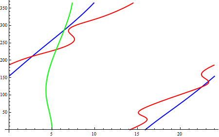
enter image description here

3 revs · Accepted Answer · 2017-04-13 12:56:07Z

The trick is to use Split in a ListPlot to introduce breaks into the data at the offending points:

Show[     
 ListPlot[
  Split[
   {astroData["RightAscension", "Mars", #, $GeoLocation], #} & /@ Range[0, 365],
   (Abs[#2[[1]] - #1[[1]]] < 20) &
   ], PlotStyle -> Blue, AspectRatio -> 1/1.6, Joined -> True],     
 ListPlot[
  Split[
   {astroData["RightAscension", "Mercury", #, $GeoLocation], #} & /@ Range[0, 365],
   (Abs[#2[[1]] - #1[[1]]] < 20) &
   ], PlotStyle -> Red, AspectRatio -> 1/1.6, Joined -> True],     
 ListPlot[
  Split[
   {astroData["RightAscension", "Jupiter", #, $GeoLocation], #} & /@ Range[0, 365],
   (Abs[#2[[1]] - #1[[1]]] < 20) &
   ], PlotStyle -> Green, AspectRatio -> 1/1.6, Joined -> True],     
 PlotRange -> {{0, 24}, {0, 365}}]

(Using a function, astroData, defined elsewhere to speed things up a bit.)

enter image description here

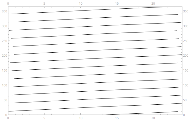
Update: While Split alone works for certain kinds of plots, it will not work for ListPlot, for which splitting will introduce a gap between the points where the lists are split, and the edges of the plot. This is not pronounced for steep lines, but is dramatic for shallow ones:

ListPlot[
 Split[
  {astroData["RightAscension", "Moon", #, $GeoLocation], #} & /@ Range[0, 365], 
  (Abs[#2[[1]] - #1[[1]]] < 20) &], 
 PlotStyle -> Black, AspectRatio -> 1/1.6, Joined -> True,
PlotRange -> {{0, 24}, {0, 365}}]

enter image description here

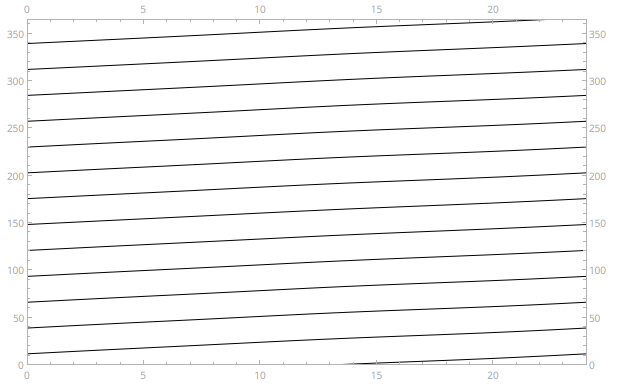
One way to overcome this is to "pad" the introduced gaps with "duplicates" of the points across the gap, shifted outside the edge of the plot. This can be done for arbitrary lists of data with something like

wrapDataList[data_, xmin_, xmax_, xgap_ ] :=
 Split[ 
  ReplaceRepeated[data, 
   {h___, {x1_, y1_}, {x2_, y2_}, t___} 
   /; (Abs[(x2 - x1)] > xgap && x2 >= xmin && x1 <= xmax) ->
     {h, {x1, y1}, {x2 + (xmax - xmin), y2}, {x1 - (xmax - xmin), y1}, {x2, y2}, t}],
  (#2[[2]] > #1[[2]]) & ]

which gives:

ListPlot[
 wrapDataList[
  {astroData["RightAscension", "Moon", #, $GeoLocation], #} & /@ Range[0, 365],
  0, 24, 20],
 PlotStyle -> Black, Joined -> True,
PlotRange -> {{0, 24}, {0, 365}}]

enter image description here

Since all of the answers (notably John's incomplete one) helped arrive at this, I'm making this CW. If someone wants to use this to improve their answer, I'll consider accepting that. Alternatively, please improve (or just vote up) this one so it can be taken as the answer. — orome, Commented Oct 8, 2012 at 23:38

John · Accepted Answer · 2012-10-08 04:37:33Z

1

I don't how your data of each of your ParametricPlot looks like, but try to adapt the following:

Split[data, #1[[2]] != #2[[2]] &]

answered Oct 8, 2012 at 4:37

John

4,4011 gold badge27 silver badges41 bronze badges

2

$\begingroup$ "I don't how your data of each of your ParametricPlot looks like..." - OP gave the code for producing the discontinuous plots. He wants the discontinuous plots to be made continuous, by stitching the two pieces together. $\endgroup$
– J. M.'s missing motivation ♦
Commented Oct 8, 2012 at 4:42
$\begingroup$ @J.M. I'm not familiar with AstronomicalData but maybe it is possible to produce the data via Table (i.e. wrapping AstronomicalData with Table) and then to use ListLinePlot with InterpolationOrder->3. $\endgroup$
– John
Commented Oct 8, 2012 at 4:50
$\begingroup$ That won't cure the problem OP has; the function itself has a (spurious) discontinuity that needs to be remedied. See this similar question. $\endgroup$
– J. M.'s missing motivation ♦
Commented Oct 8, 2012 at 5:09

Add a comment |

b.gates.you.know.what · Accepted Answer · 2012-10-08 07:45:49Z

1

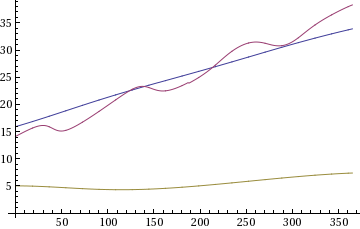
One way is to first use Clip to keep all differences between consecutive data points within a given range, then reconstruct the list using Accumulate:

dataMars =  Table[{d, AstronomicalData["Mars", {"RightAscension", 
 DatePlus[Date[], 
  d], {$GeoLocation[[1]], $GeoLocation[[2]]}}]}, {d, 0, 365}]

dataFixed[data_, minDiff_, maxDiff_] := With[{diff = Differences[data[[All, 2]]]}, 
  Transpose[{data[[All, 1]], Accumulate[
    Join[{data[[1, 2]]}, Clip[diff, {minDiff, maxDiff}]]]}]]

dataMars2 = dataFixed[dataMars, 0.0394, 0.0559];
dataMercury2 = dataFixed[dataMercury, -0.08668, 0.1493437];
dataJupiter2 = dataFixed[dataJupiter, -0.00969, 0.01664];

ListLinePlot[{dataMars2, dataMercury2, dataJupiter2}]

enter image description here

edited Oct 8, 2012 at 7:45

answered Oct 8, 2012 at 6:50

b.gates.you.know.what

20.2k2 gold badges45 silver badges86 bronze badges

$\begingroup$ This isn't what the figure should look like. See my clarification and the figure in fizzics answer. $\endgroup$
– orome
Commented Oct 8, 2012 at 13:35

Add a comment |

Stack Exchange Network

How do I get rid of a "jump" in my plot?

7 Answers 7

Your Answer

Not the answer you're looking for? Browse other questions tagged
plotting
or ask your own question.

Linked

Hot Network Questions

How do I get rid of a "jump" in my plot?

7 Answers 7

Your Answer

Sign up or log in

Post as a guest

Not the answer you're looking for? Browse other questions tagged plotting or ask your own question.

Linked

Related

Hot Network Questions

Not the answer you're looking for? Browse other questions tagged
plotting
or ask your own question.