Dynamical system problem x(t+1) = Ax(t)

Question

I have a problem that have been trying to solve but it's not going so good. I would like some guidelines on how to work myself around this problem:

Two neighboring countries spy on each other and adapt its defense budget against each other depending on the situation in the neighborhood. Let country A's annual defense budget be a(t) (in billion) and country B's b(t). The change in budget changes each year according to the relationship:

a (t + 1) = r a (t) + s B (t)

b (t + 1) = s a (t) + r b (t)

where r is a positive number a bit less than 1 and s is a small postive number a bit greater than 0. Suppose that r is greater than s, that is, r>s. The budget for the two countries can be described by the vector x (t) = (a b) (<--- matrix) where a = a(t) and b = b(t)

If a(0) = 30 and b(0) = 5, what will happen with both the countries defense budget in the long run?

Solve tasks a) to e) both on paper and in Mathematica.

a) Set up the system transition matrix A such that x(t + 1) = Ax(t)

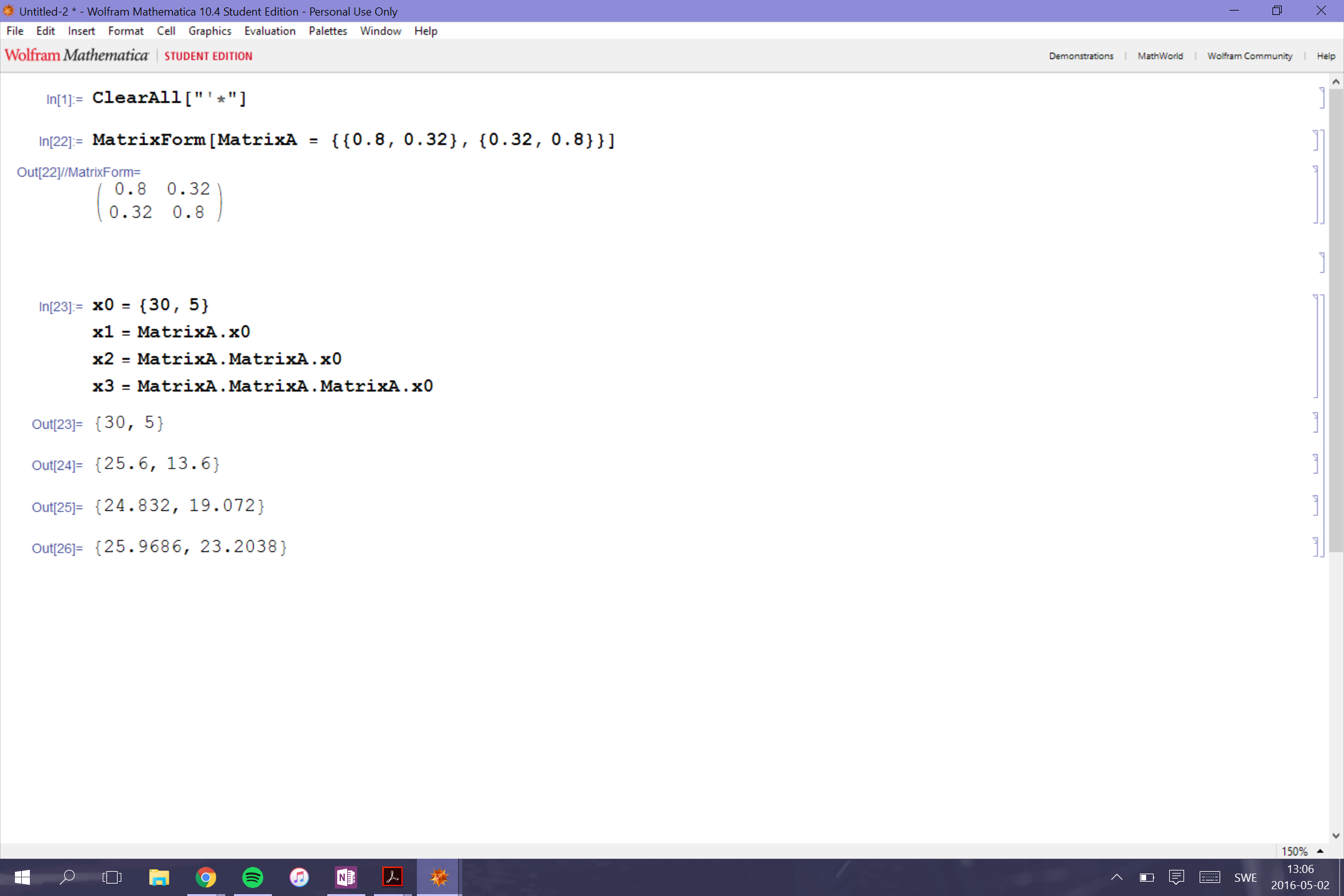
So what I've done so far is to select r = 0.8 and s = 0.32 and defined it as a 2x2 matrix and I've also defined a column vector with a(0)=30 and b(0)=5, so what I have in mathematica right know is:

I don't feel like this is how I'm supposed to do. At least this doesn't feel like how it should turn out in the "long run".

I would be very happy for someone to help/guide me through this! Thank you!

EDIT: I solved the problem and would like to have some feedback on how it is, if it's messy to follow. I would be thankful! :)

2nd EDIT: In my second question I need to find the Eigenvalues, Eigenvectors and Eigenbase. I have calculated by hand and I've gotten the Eigenvalues to lamda=1 and lamda=0.8 (when using the matrix {0.9,0.1},{0.1,0.9}) and the v1 = {1,1} and v2 = {-1,1}..I've gotten the right answers for it also on mathematica:

MatrixA = {{0.9, 0.1}, {0.1, 0.9}};
EigenMatrix = {{lm, 0}, {0, lm]}};
detMatrix = MatrixA - EigenMatrix
{{0.9 - lm], 0.1}, {0.1, 0.9 - lm}}

KarEk = Det[detMatrix]
0.8 - 1.8lm + lm^2
LamdaVarden = Roots[KarEk == 0, lm]
lm == 0.8 || lm == 1.

However, when trying to solve the Eigenvectors I get:

Eigenvectors[{{0.9, 0.1}, {0.1, 0.9}}]
{{0.707107, 0.707107}, {-0.707107, 0.707107}}

This is wrong, what am I doing wrong?

Answer 1

x[t_] = {a[t], b[t]} /. RSolve[{
     a[t + 1] == r*a[t] + s*b[t],
     b[t + 1] == s*a[t] + r*b[t],
     a[0] == 30, b[0] == 5}, {a[t], b[t]}, t][[1]]

Since 0 < s < r < 1 then 0 < r - s < 1 - s < 1 and for large t, (r -s)^t is approximately zero.

 x[t] /. (r - s)^t -> 0

i.e., a[t] ≈ b[t] for large t

Plot[
 Evaluate[{
   x[t] /. {r -> 0.8, s -> 0.32},
   x[t] /. {r -> 0.68, s -> 0.32},
   x[t] /. {r -> 0.6, s -> 0.32}}],
 {t, -1, 20},
 PlotStyle ->
  (AbsoluteDashing /@ {{7, 3}, {7, 7}}),
 Frame -> True, Axes -> False,
 PlotLegends -> {
   "a[t], r+s=1.12", "b[t], r+s=1.12",
   "a[t], r+s=1", "b[t], r+s=1",
   "a[t], r+s=0.92", "b[t], r+s=0.92"},
 Epilog -> {Text["r + s = 1.12", {13, 100}],
   Text["r + s = 1", {13, 35/2}, {0, -1.5}],
   Text["r + s = 0.92", {13, 0}, {0, .5}]}]

In the limit,

Piecewise[
 Assuming[{0 < r < 1, 0 < s < 1, s < r, #},
    {Limit[x[t], t -> Infinity], #}] & /@
  {r + s < 1, r + s == 1, 
   r + s > 1}]

x /@ Range[0, 10] /. {r -> 0.8, s -> 0.32} // Column

EDIT: For the generic solution

Format[a0] := Subscript[a, 0]
Format[b0] := Subscript[b, 0]

x1[t_] = {a[t], b[t]} /. RSolve[{
      a[t + 1] == r*a[t] + s*b[t],
      b[t + 1] == s*a[t] + r*b[t],
      a[0] == a0, b[0] == b0},
     {a[t], b[t]}, t][[1]] // Simplify

x2[t_] = MatrixPower[{{r, s}, {s, r}}, t].{a0, b0} // Simplify;

As J.M. pointed out in a comment, this can also be written as

x2[t_] = MatrixPower[{{r, s}, {s, r}}, t, {a0, b0}] // Simplify;

x1 and x2 are identical

x1[t] === x2[t]

(*  True  *)

Approximate solution for large values of t

xApprox[t_] = Simplify[x1[t] /. (r - s)^t -> 0]

a[t] and b[t] are approximately equal for large t (and identical in the limit)

Equal @@ xApprox[t]

(*  True  *)

In the limit,

Piecewise[
 Assuming[
    {0 < r < 1, 0 < s < 1, s < r, a0 > 0, b0 > 0, #},
    {Limit[x1[t], t -> Infinity], #}] & /@
  {r + s > 1, r + s == 1, 
   r + s < 1}]

Answer 2

The way to answer this generically is via eigenvalues. Set up your matrix and take its eigenvalues:

mat = {{r, s}, {s, r}};
Eigenvalues[mat]

{r - s, r + s}

If either r-s or r+s is greater than 1 (in magnitude) then the system will be unstable. If both are less than one, it will decay to zero. For your values r=0.8 and s=0.32, you have instability, which is why you see the numerical simulations diverge.