Solving wave PDE

Question

I am trying to solve the wave PDE with NDSolve. Below is the equation:

NDSolve[{D[u[x, t], {t, 2}] == 2*D[u[x, t], {x, 2}], u[0, t] == 0, 
u[10, t] == 0, u[x, 0] == 5, D[u[x, 0] == 0]}, 
u[x, t], {x, 0, 10}, {t, 0, 5}]

When I try to get the solution I get the following error:

NDSolve::ibcinc: Warning: boundary and initial conditions are inconsistent.

NDSolve::ndinpd: The initial conditions did not evaluate to an array of numbers of depth 1 on the spatial grid. Initial conditions for partial differential equations should be specified as scalar functions of the spatial variables.

My Boundary conditions are:

• when x=0 (at t=0) is zero
• when x=10 (at t=0) is also zero

My Initial conditions are:

• u when $t=0$ g[x]=5
• derivative of u when t=0 is zero

By this initial condition it means the string is stretched in vertical direction by 5 units at its center, initial velocity being zero and then let go.

I want to check the wave pattern of the string with these conditions.

Answer 1

There are two different methods for solving the OP"s problem :

• The Method of Lines with the option "SpatialDiscretization" -> {"TensorProductGrid"...

• The Method of Lines with the option "SpatialDiscretization" -> {"FiniteElement"}. This solution is the Mathematica 10 implementation of the Finite Element Method for transcient PDEs.

In both cases the Method of Lines does the temporal integration.

Apart from this, the solution will be given for the following cases :

1) OP's equation and initial condition u[x,0] == triangle : u[x,0] == 5 - Abs[x-5] :

2) Because the exact OP's equation doesn't give a realistic result, the equation is modified by adding some loss and the result is shown

3) initial condition : u[x,0] == 5 :

1) initial condition u[x,0] == triangle, Lossless

Method of Lines with TensorProductGrid

solTensorLossless = 
  NDSolve[{D[u[x, t], {t, 2}] == 2*D[u[x, t], {x, 2}], u[0, t] == 0, 
     u[10, t] == 0, 
     u[x, 0] == 5 - Abs[x - 5], (D[u[x, t], t] /. t -> 0) == 0}, 
    u, {x, 0, 10}, {t, 0, 15}, 


 Method -> {"MethodOfLines", "TemporalVariable" -> t, 
      "SpatialDiscretization" -> {"TensorProductGrid", 
        "MinPoints" -> {50}, "MaxPoints" -> {100}, 
        "DifferenceOrder" -> "Pseudospectral"}}][[1, 1, 2]];

Table[Labeled[
    Plot[solTensorLossless[x, t], {x, 0, 10}, 
     PlotRange -> {Automatic, {-5, 5}}], t], {t, 0, 15, 0.2}]  // 
  Export["TensorLossLess.gif", #] &;

SystemOpen["TensorLossLess.gif"] 

Method of Lines with Finite Elements

solFEMLossless = 
  NDSolve[{D[u[x, t], {t, 2}] == 2*D[u[x, t], {x, 2}], u[0, t] == 0, 
     u[10, t] == 0, 
     u[x, 0] == 5 - Abs[x - 5], (D[u[x, t], t] /. t -> 0) == 0}, 
    u, {x, 0, 10}, {t, 0, 15}, 
    Method -> {"MethodOfLines", "TemporalVariable" -> t, 
      "SpatialDiscretization" -> {"FiniteElement"}}][[1, 1, 2]];

Table[Labeled[
    Plot[solFEMLossless[x, t], {x, 0, 10}, 
     PlotRange -> {Automatic, {-5, 5}}], t], {t, 0, 15, 0.2}]  // 
  Export["FEMLossLess.gif", #] &;

SystemOpen["FEMLossLess.gif"]

2) initial condition u[x,0] == triangle, Lossy

Method of Lines with TensorProductGrid

solTensorLossy = 
  NDSolve[{D[u[x, t], {t, 2}] + 0.3 D[u[x, t], {t, 1}] == 
      2*D[u[x, t], {x, 2}], u[0, t] == 0, u[10, t] == 0, 
     u[x, 0] == 5 - Abs[x - 5], (D[u[x, t], t] /. t -> 0) == 0}, 
    u, {x, 0, 10}, {t, 0, 15}, 
    Method -> {"MethodOfLines", "TemporalVariable" -> t, 
      "SpatialDiscretization" -> {"TensorProductGrid", 
        "MinPoints" -> {50}, "MaxPoints" -> {100}, 
        "DifferenceOrder" -> "Pseudospectral"}}][[1, 1, 2]];

Table[Labeled[
    Plot[solTensorLossy[x, t], {x, 0, 10}, 
     PlotRange -> {Automatic, {-5, 5}}], t], {t, 0, 15, 0.2}]  // 
  Export["TensorLossy.gif", #] &;

SystemOpen["TensorLossy.gif"]

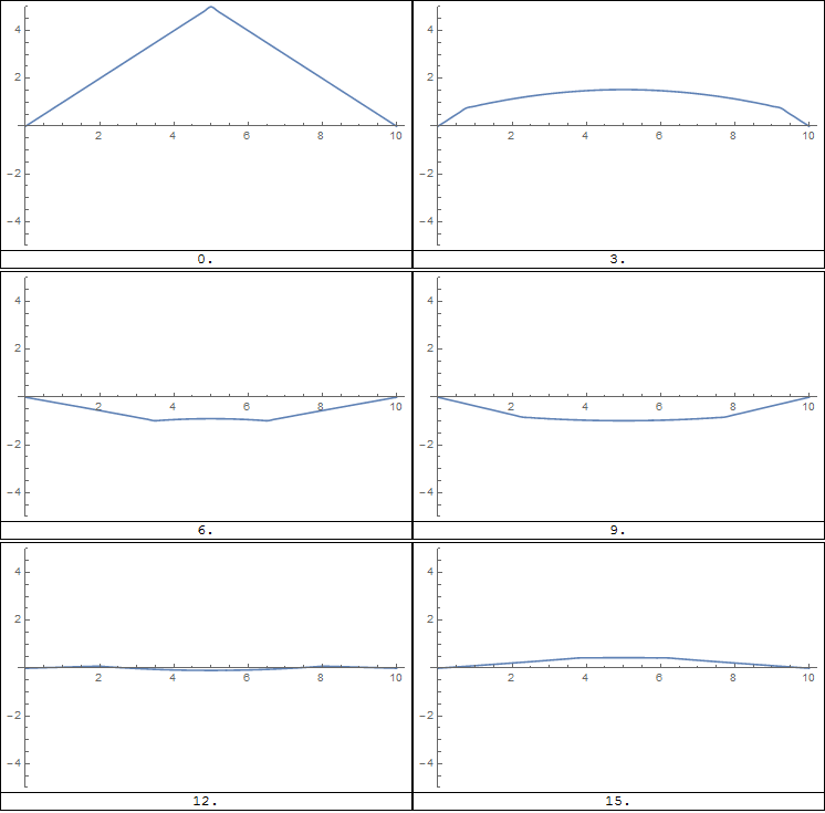
Method of Lines with Finite Elements

solFEMLossy = 
  NDSolve[{D[u[x, t], {t, 2}] + 0.3 D[u[x, t], {t, 1}] == 
      2*D[u[x, t], {x, 2}], u[0, t] == 0, u[10, t] == 0, 
     u[x, 0] == 5 - Abs[x - 5], (D[u[x, t], t] /. t -> 0) == 0}, 
    u, {x, 0, 10}, {t, 0, 15}, 
    Method -> {"MethodOfLines", "TemporalVariable" -> t, 
      "SpatialDiscretization" -> {"FiniteElement"}}][[1, 1, 2]];

Table[Labeled[
    Plot[solFEMLossy[x, t], {x, 0, 10}, 
     PlotRange -> {Automatic, {-5, 5}}], t], {t, 0, 15, 0.2}]  // 
  Export["FEMLossy.gif", #] &;

SystemOpen["FEMLossy.gif"]

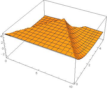
3) initial condition : u[x,0] == 5

Method of Lines + TensorProductGrid

solTensorProductGrid00 = 
  NDSolve[{
          D[u[x, t], {t, 2}] == 2*D[u[x, t], {x, 2}], 
          u[0, t] == 0, 
          u[10, t] == 0,
          u[x, 0] == 5,
          (D[u[x, t], t] /. t -> 0) == 0
         }, 
         u,
         {x, 0, 10}, {t, 0, 5}, 
         Method -> {"MethodOfLines",
                    "TemporalVariable" -> t, 
                    "SpatialDiscretization" -> {"TensorProductGrid", 
                                                "MinPoints" -> {50},
                                                "MaxPoints" -> {100},
                                                "DifferenceOrder" ->"Pseudospectral" 
                                               }
                   }
        ];

solTensorProductGrid = solTensorProductGrid00[[1, 1, 2]];

Plot3D[solTensorProductGrid[x, t], {x, 0, 10}, {t, 0, 5}]

Method of Lines + Finite Element

solFiniteElementMethod00 = 
 NDSolve[{
         D[u[x, t], {t, 2}] == 2*D[u[x, t], {x, 2}],
         u[0, t] == 0, 
         u[10, t] == 0,
         u[x, 0] == 5,
         (D[u[x, t], t] /. t -> 0) == 0
         }, 
         u,
         {x, 0, 10}, {t, 0, 5}, 
         Method -> {"MethodOfLines",
                    "TemporalVariable" -> t, 
                    "SpatialDiscretization" -> {"FiniteElement"}}
        ]

solFiniteElementMethod = solFiniteElementMethod00[[1, 1, 2]];

Plot3D[solFiniteElementMethod[x, t], {x, 0, 10}, {t, 0, 5}]

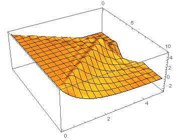
Note : the theorical solution is : two perfect steps propagating from the edges towrad center (hyperbolic PDEs propagate discontinuities). Here the steps are not perfect since we dont have u[0,t]=u[10,t]=0

My version of Mathematica : 10.0.2.0 Windows 64 bits