5
$\begingroup$

I would like to estimate the parameters of a derived distribution fSurvivalGompertzNoiseDist below.

This distribution represents simulations from a probability distribution that has the same shape as a Gompertz survival function, with noise added. Basically, I am sampling from a population whose population age structure is given by a Gompertz-survival function. (Individual age follows a Gompertz distribution, and assuming a constant rate of birth into the population, this results in a Gompertz-survival function for population age structure.) The gaussian noise represents measurement error.

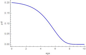
I want to estimate the parameters of the underlying Gompertz function (which I call α and β below) by sampling from the population. As I said, to be clear, this population follows a Gompertz-survival age distribution, not a Gompertz distribution (that is for the individual age). It looks something like:

enter image description here

So first I define my population distribution fSurvivalGompertzNoiseDist:

fSurvivalGompertzDist[α_, β_] := 
    ProbabilityDistribution[
      (1/((E^(α/β) Gamma[0, α/β])/β)E^(((1 - E^(t β)) α)/β)),
      {t, 0, ∞},
      Assumptions -> {α > 0, β > 0}
     ]

fSurvivalGompertzNoiseDist[α_, β_, σ_] := 
      TransformedDistribution[u + v, {u \[Distributed] fSurvivalGompertzDist[α, β], v \[Distributed] NormalDistribution[0, σ]}]

I then use a slightly-differently defined distribution to generate independent samples (I simply omit the assumptions in the above):

    fSurvivalGompertzDistRand[α_, β_] := 
     ProbabilityDistribution[
       (1/((E^(α/β) Gamma[0, α/β])/β) E^(((1 - E^(t β)) α)/β)),
       {t, 0, ∞}
      ]

fSurvivalGompertzNoiseDistRand[α_, β_, σ_] := 
      TransformedDistribution[u + v, {u \[Distributed] fSurvivalGompertzDistRand[α, β], v \[Distributed] NormalDistribution[0, σ]}]

data = RandomVariate[fSurvivalGompertzNoiseDistRand[0.016, 0.65, 1], {100}];

I then try to use FindDistributionParameters on this:

FindDistributionParameters[data, fSurvivalGompertzNoiseDist[α, β, σ]]

Which returns the following error:

The support of the distribution TransformedDistribution...could not be determined.

The validity of the data for TransformedDistribution...could not be determined.

I have tried removing the assumptions above, as well as adding them to the transformed distribution function. I have also tried specifying σ > 0 in the transformed distribution function. None of these seems to make any difference.

Finally, I also tried to manually calculate the LogLikelihood for the fSurvivalGompertzNoiseDist, but this returns back an unevaluated result. I have also tried to find the PDF (using Mathematica's $PDF$), which again returns back an unevaluated result.

Does anyone have an idea as to how I can make some headway here? As well as finding the answer, speed is of the essence, as I will need to do this calculate thousands of times. I know I have Jim's answer below, but this method is sensitive to parameter initial values. So for example, $\alpha=0.1,\beta=0.0001$, the method takes a long time, and can result in fairly imprecise estimates.

edit: I can calculate the characteristic function of the distribution, but this doesn't seem to yield moments in a simple enough form to think about doing method-of-moments estimation. Specifically the characteristic function is:

$\frac{e^{-\frac{1}{2} \sigma ^2 t^2} \left(\frac{\alpha }{\beta }\right)^{-\frac{i t}{\beta }} \left(\Gamma \left(\frac{i t}{\beta },\frac{\alpha }{\beta }\right)-\Gamma \left(\frac{i t}{\beta }\right)\right)}{\Gamma \left(0,\frac{\alpha }{\beta }\right)}$

I have also tried to estimate the moment generating function, but Mathematica doesn't seem to be able to do this.

edit 2: It does occur to me that, if I can't find the likelihood here, but can generate independent samples from the distribution, I could do a type of approximate Bayesian computation. Essentially I only need point estimates of the parameters, so could do a sort of least squared fitting between the actual data and the simulated. However, this would be expensive; only to be resorted to if there isn't an easier way.

edit 3: I have now managed to determine the mean and variance of the distribution. This is because $Z=X+Y$, where $X\sim fSurvivalGompertzDist[\alpha,\beta]$, and $Y\sim N(0,\sigma)$ are independent. Due to this independence I can calculate the mean, and variance of each separately, and add them to get what I want:

mean = MeijerG[{{}, {1, 1}}, {{0, 0, 
   0}, {}}, α/β]/(β Gamma[0, α/β])

variance = -((MeijerG[{{}, {1, 1}}, {{0, 0, 0}, {}}, α/β]^2 - 
        2 Gamma[0, α/β] MeijerG[{{}, {1, 1, 1}}, {{0, 0, 0, 
        0}, {}}, α/β])/(β^2 Gamma[
        0, α/β]^2)) + σ^2

However, current attempts to use these with $NSolve$, $FindRoot$ etc. along with the empirical moments have failed: each function just returns the eqn. I am trying to solve unevaluated.

edit 4: I have tried to use the characteristic function, and its empirical analogue: $ecf=\frac{1}{n} \sum_{i=1}^n exp(t i X_i)$ to do a sort of method of moments as in the paper: http://www.mysmu.edu/faculty/yujun/research/yuer.pdf but I don't seem to get reasonable estimators out unfortunately.

edit 5: Since I am able to generate independent samples from this distribution, I have tried comparing the mean and variance of my distribution with that from the random samples. I do that using this function:

fCompareMeanVar[aMean_, aVar_, α_, β_, σ_, aNumComparisons_] := 
 Module[{data = 
    RandomVariate[fSurvivalGompertzNoiseDistRand[α, β, [Sigma]], \{aNumComparisons}], bMean, bVar}, bMean = Mean@data; 
    bVar = Variance@data; Total@ {aMean - bMean, aVar - bVar}^2]

Unfortunately, the following doesn't seem to work.

NMinimize[{fCompareMeanVar[Mean@data, 
   Variance@data, α, β, 1, 1000], 1 > α > 0, 
   1 > β > 0}, {α, β}, 
   Method -> "SimulatedAnnealing", AccuracyGoal -> 1]

Best,

Ben

$\endgroup$
5
  • 1
    $\begingroup$ I wonder why you are adding in Gaussian random noise. This gives you data with negative ages. Might a multiplicative error structure be better? $\endgroup$
    – JimB
    Commented Feb 22, 2016 at 19:46
  • $\begingroup$ @JimBaldwin Good question. However, this additive gaussian age structure is actually something that is fixed - I cannot change it. I didn't include information in the question, but it is because I am using an existing manufacturer-based machine learning algorithm to estimate the age of individuals I sample from the population. Not my choice, but a necessity here, I'm afraid. Best, Ben $\endgroup$
    – ben18785
    Commented Feb 22, 2016 at 19:49
  • $\begingroup$ So what do you do with the negative data? About 8% of your example data is negative. That doesn't detract from the desire or the ability to get estimates of the parameters but it does call into question the appropriateness of the model for real-life data. (But maybe the setting of $\sigma=1$ is too much noise and is only for giving specificity to an example.) $\endgroup$
    – JimB
    Commented Feb 22, 2016 at 19:57
  • $\begingroup$ @JimBaldwin Thanks for your comment. I don't want to really get into the details here, as it is not important for the question itself, to be honest. Basically, it is actually beneficial to sometimes pick a negative age, since for us, the most important thing is minimising bias in our estimators. If we were to make all the negative points zero, this biases our mean estimates, which is problematic. The value of $\sigma=1$ I state above is realistic, and don't need to change it. Not sure that helps answer your question! Best, Ben $\endgroup$
    – ben18785
    Commented Feb 22, 2016 at 20:00
  • 1
    $\begingroup$ While there are a lot of folks that do think that minimizing bias is "the most important thing", you might want sometimes to think otherwise. As in your example, I'd certainly accept some bias if my estimator did not produce nonsense values. (And there are practical situations, too, where a little bias can considerably result in a much smaller mean square error.) It's not that unbiasedness is bad. It's just not the only thing. $\endgroup$
    – JimB
    Commented Feb 28, 2016 at 19:22

2 Answers 2

5
$\begingroup$

Here's a brute force method of moments approach. First define the theoretical moments:

(* Check on density integrating to 1 *)
totalProb = Integrate[(E^(-(α/β) + ((1 - E^(x β)) α)/β) β)/Gamma[0, α/β], {x, 0, ∞},
  Assumptions -> {α > 0, β > 0}]

(* Mean, variance, and 3rd central moment of sum of Gompertz survival 
   plus Gaussian noise (yuk!) *)
mean = 0 + Integrate[x (E^(-(α/β) + ((1 - E^(x β)) α)/β) β)/Gamma[0, α/β], {x, 0, ∞},
   Assumptions -> {α > 0, β > 0}]
variance = σ^2 + Integrate[x^2 (E^(-(α/β) + ((1 - E^(x β)) α)/β) β)/ Gamma[0, α/β], {x, 0, ∞},
   Assumptions -> {α > 0, β > 0}] - mean^2

thirdCentralMoment = 2 mean^3 - 3 mean (variance - σ^2 + mean^2) +
  Integrate[x^3 (E^(-(α/β) + ((1 - E^(x β)) α)/β) β)/Gamma[0, α/β], {x, 0, ∞}, 
   Assumptions -> {α > 0, β > 0}]

Generate some data:

data = RandomVariate[fSurvivalGompertzDistRand[0.016, 0.65], 1000] + 
   RandomVariate[NormalDistribution[0, 1], 1000];

Then calculate the corresponding sample moments:

(* Get sample mean, variance, and central third moment *)
xbar = Mean[data];
s2 = Variance[data];
cm3 = CentralMoment[data, 3];

Now we have 3 equations and 3 unknowns:

(* Solve using method of moments: equating some sample moments to theoretical moments *)
FindRoot[{mean == xbar, variance == s2, thirdCentralMoment == cm3},
 {{α, 0.2}, {β, 0.65}, {σ, 1}}]
(* {α->0.01993564678419563, β->0.5975162143103656, σ->1.0505200325360906} *)

You might also need some good initial values for the parameters.

$\endgroup$
8
  • $\begingroup$ Thanks! I was about to post my solution when you posted yours. Mine is pretty much the same, although is a bit slower (using $FindMinimum$ instead of $FindRoot$). However, one benefit is that it doesn't depend on initial parameters. Unfortunately, it looks like doing these types of calculation thousands of times will be very hard. Unless someone comes in with a better solution. Thanks again here! Best, Ben $\endgroup$
    – ben18785
    Commented Feb 22, 2016 at 23:01
  • 2
    $\begingroup$ Good. It was clear that as you updated you weren't just sitting around. Not needing initial values is a good thing until it isn't. $\endgroup$
    – JimB
    Commented Feb 22, 2016 at 23:18
  • $\begingroup$ If it interests you, I was also looking at this paper: mysmu.edu/faculty/yujun/research/yuer.pdf that looks at using the empirical characteristic function to do method of moments. Not sure if it'll work here, but thought it was interesting nonetheless. Best, Ben $\endgroup$
    – ben18785
    Commented Feb 22, 2016 at 23:27
  • 2
    $\begingroup$ I think it's OK. If the third central moment is $E((u+v-mean)^3)$, then we can get that by expanding what's in parentheses and applying a few replacement rules to do what the expectation operator does: (Expand[(u + v - mean)^3]) /. {v^3 -> 0, v^2 -> \[Sigma]^2, v -> 0, u^3 -> Eu3, u^2 -> variance - \[Sigma]^2 + mean^2, u -> mean} which equals Eu3 + 2 mean^3 - 3 mean (mean^2 + variance - \[Sigma]^2). $\endgroup$
    – JimB
    Commented Feb 27, 2016 at 22:00
  • 1
    $\begingroup$ I'm not assuming that v^3 = 0, I'm knowing that E[v^3] = 0 (given that the mean is zero for v). A normal distribution is symmetric and all of the odd central moments of a normal are zero. And I've matched the theoretical central 3rd moment with the sample central 3rd moment to get the 3rd equation. $\endgroup$
    – JimB
    Commented Feb 28, 2016 at 0:32
1
$\begingroup$

I have now reached an answer with which I am happy. It is basically the result on tinkering with Jim Baldwin's answer (thanks again Jim!)

After calculating the mean, variance and third central moments as per Jim's method, the result is given in terms of the Meijer $G$ function. As Jim suggests, these three moments can then be set equal to their sample equivalents, and solved for the parameter estimates.

The problem with the use of the Meijer $G$ results is that they are slow, and I also found that Mathematica's solvers to be very sensitive to their starting points.

However, when I used FunctionExpand on each of the results, this yielded expressions that were much more amenable to the solvers. For example, for the mean I got:

FunctionExpand[mean] = (EulerGamma^2/2 + π^2/12 - (α    HypergeometricPFQ[{1, 1, 
                  1}, {2, 2, 2}, -(α/β)])/β + 
                  EulerGamma Log[α/β] + 
                  1/2 Log[α/β]^2)/(β (-ExpIntegralEi[-(α/\
                  β)] - Log[α/β] + 
                  1/2 (Log[-(α/β)] - Log[-(β/α)])))

I decided to also use NMinimize to look for solutions, since I wanted a solver that didn't depend on start point. I defined functions for each of the expanded moments, and took the square of the difference of the moment from its sample equivalent:

fEstimateParameters[aMean_, aVar_, aThird_] := 
              FindMinimum[{Total[{mean[α, β] - aMean, 
              var[α, β, σ] - aVar, 
              thirdCM[α, β, σ] - aThird}^2], 
              1 > α > 0 && 
              1 > β > 0.05 && σ > 0}, {α, β, σ}

Generating my data using a function I define in the question, and using the above to solve for the parameters:

data = RandomVariate[fSurvivalGompertzNoiseDistRand[0.016, 0.65, 1], {100}];
fEstimateParameters[Mean@data, Variance@data, CentralMoment[#, 3] &@data] // Timing

I get the results:

{0.536002, {0.15919, {α -> 0.0874638, β -> 0.401905, σ -> 1.10882}}}

The above function seemed to work well for the majority of cases. For very low $\beta$ values, there are problems, but these are just due to the lack of identification of $\alpha$ and $\beta$.

Best,

Ben

$\endgroup$

Your Answer

By clicking “Post Your Answer”, you agree to our terms of service and acknowledge you have read our privacy policy.

Not the answer you're looking for? Browse other questions tagged or ask your own question.