How to make a Line[] with no end?

Question

I'm trying to do this:

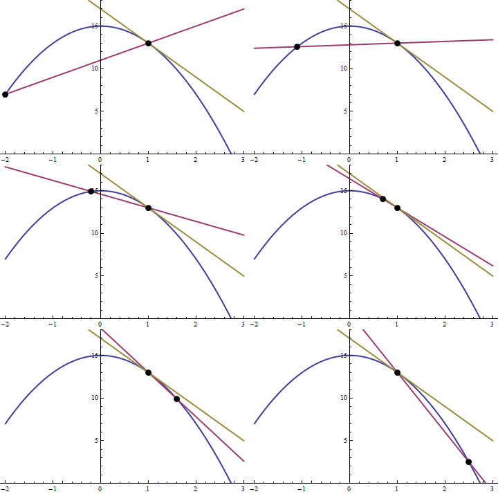
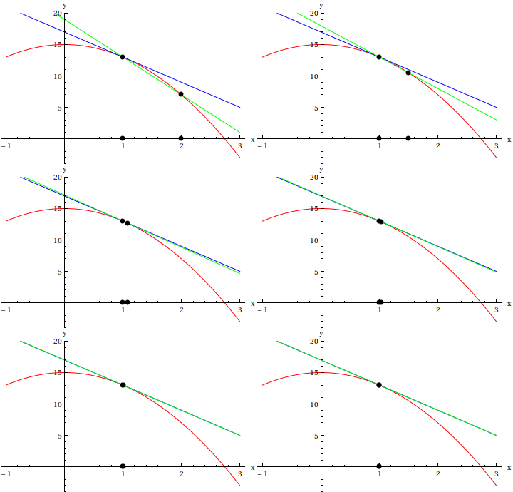
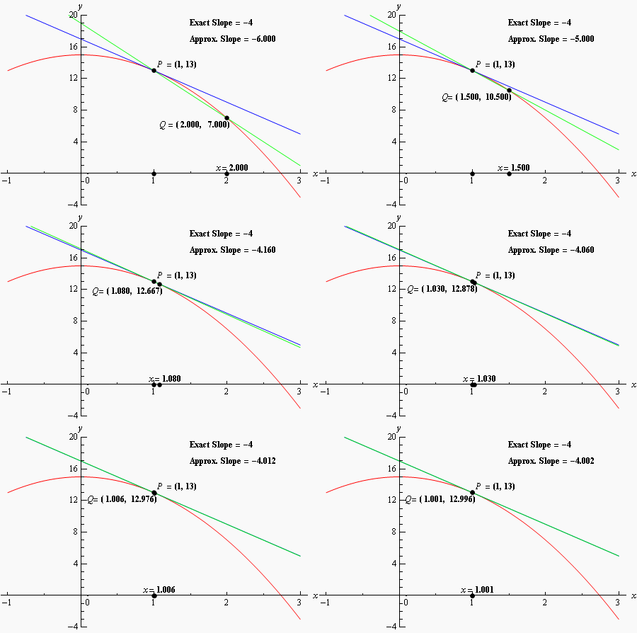
In this graph, the secant points are aproximated in order to become the tangent, it seems I need some kind of function which plots a line based on two points and it's points do not limit the end of the line.

This is what I could do, as you can evaluate (see?), you'll see the line ends at the proposed points.

Show[{
  Plot[{15 - 2 x^2}, {x, -1, 3}],
  Graphics[Line[{{1, 13}, {2, 7}}]]
  }]

I've read the reference on line but I still have no idea on how to do it, I imagine there are two ways of doing it, (1) the way I did, with Line; (2) With the Plot function.

Answer 1

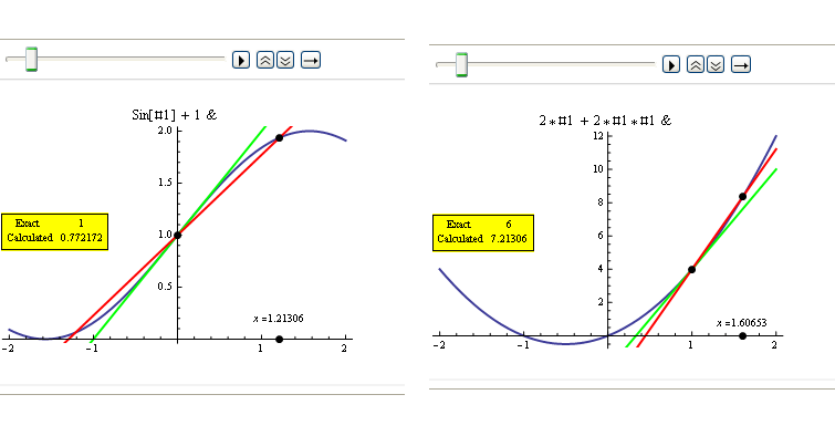
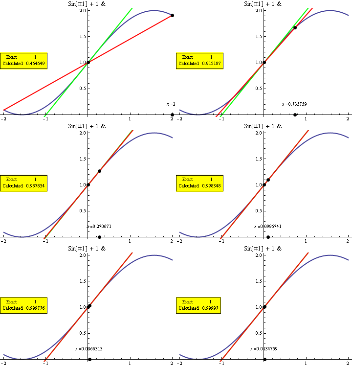
A little bit more general (for any function, interval, starting and final points...) and implementing most of your labels:

appDeriv[f_, x0_, xinit_, pRange_List] := Module[{xseq, tan, tan1, l, plot, absPR},
   xseq      = Table[x0 + Exp[-n/2] (xinit - x0), {n, 0, 10}]; (* exploration points *)
   tan       = D[f@x, x] /. x -> x0;                           (* real derivative *)
   tan1[x_] := (f[x] - f[x0])/(x - x0);                        (* approx derivative  *)
   l[t_]    := Line[Transpose[{pRange, pRange t + (-t x0 + f@x0)}]]; (*line w/given angle*)
   plot = Plot[f@x, {x, pRange[[1]], pRange[[2]]}, PlotStyle->Thick, PlotLabel->InputForm@f];
   absPR = AbsoluteOptions[plot, PlotRange][[1, 2]];     (*get actual prange for the plot*)
 Animate[Show[
  plot,
  Graphics[{
    Thick, PointSize[Large],
    Green, l[tan], Red, l[tan1[p]], Black,  (* The two lines *)
    Point[{x0, f@x0}],Point[{p,AbsoluteOptions[plot, AxesOrigin][[1,2,2]]}], Point[{p, f@p}],
    Inset[ "x =" <> ToString@N@p, {p, (absPR[[2, 1]] 9 + absPR[[2, 2]])/10}],
    Inset[Framed@Grid[{{"Exact ", tan}, {"Calculated", N@tan1[p]}}], {Left,Center}, 
          {Left, Center}, Background -> Yellow]}]], 
 {p, xseq}] ];
GraphicsGrid[{{appDeriv[Sin@# + 1 &, 0, 2, {-2, 2}],appDeriv[2 # + 2 # # &, 1, 2, {-2, 2}]}}]

Answer 2

line[x_] := Solve[{a + b == 13, a x + b == 15 - 2 x^2}, {a, b}] // Quiet
f[x_, x0_] := {15 - 2 x^2, (a x + b) /. line[x0]}

Animate[ Plot[{f[x, x0], -4 x + 17}, {x, -2, 3}, PlotRange -> {0, 18}, PlotStyle -> Thick,
               Evaluated -> True, Epilog -> {PointSize[0.025], 
               Point[{{1, 13}, {x0, 15 - 2 x0^2}}]}],           {x0, -2, 2.5}]

Adding any formulae has been left up to you.

Answer 3

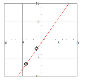
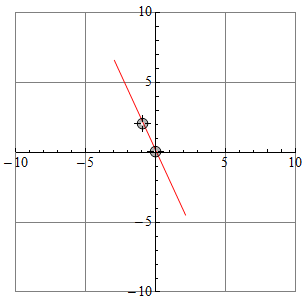
Update: version 10 introduced InfiniteLine:

DynamicModule[{pt = {{1, 1}, {2, 1}}}, 
 LocatorPane[Dynamic @ pt, 
  Graphics[{Red, Dynamic @ InfiniteLine @ pt}, PlotRange -> {{-10, 10}, {-10, 10}}, 
   Axes -> True, GridLines -> Automatic], ImageSize -> 300]]

---

It seems to me that you are asking for a way to extend a line segment specified by two points. Here is one method you might use.

extend[x:{a_, b_}, d_] := (d/Norm[a - b]) (x - {b, a}) + x

This will extend a line segment a b by distance d in either direction. Example:

DynamicModule[{pt = {{1, 1}, {2, 1}}},
 LocatorPane[Dynamic @ pt,
  Graphics[
   {Red, Line @ Dynamic @ extend[pt, 5]},
   PlotRange -> {{-10, 10}, {-10, 10}},
   Axes -> True,
   GridLines -> Automatic
  ]
 ]
]

Answer 4

f[x_] := 15 - 2 x^2

x0 = 1;
tangentLine[x_] = Normal[Series[f[x], {x, x0, 1}]]

secantLine[h_, x_] := InterpolatingPolynomial[{{x0, f[x0]}, {h, f[h]}}, x]

Animate[Plot[{f[x], tangentLine[x], secantLine[h, x]}, {x, -1, 3}, 
  AxesLabel -> {"x", "y"}, 
  Epilog -> {AbsolutePointSize[7], Point[{{x0, 0}, {x0, f[x0]}, {h, 0}, {h, f[h]}}]}, 
  PlotRange -> {-4, 20}, PlotStyle -> {Red, Blue, Green}],
  {h, Range[2., 1.1, -.1] ~Join~ Range[1.09, 1.01, -.01] ~Join~ Range[1.009, 1.001, -.001]}]

Adding the labels is up to you (hint: modify the setting of Epilog by adding Text[] primitives).

Answer 5

The purpose of this answer is to give simple, clear answers to the simple component questions,

• How to draw an infinite tangent line?
• How to draw an infinite secant line?

I will use the V10+ InfiniteLine, which Mr.Wizard has already pointed out as a way to draw an infinite line. See also the Note below.

How to draw a tangent line

Round about the eighth example under "Applications" in the documentation for InfiniteLine, one finds how to draw tangent lines to parametric plots. The example can be adapted to Plot[f[x], {x, a, b}]. The tangent line at x == x0 is given by

InfiniteLine[{x0, f[x0]}, {1, f'[x0]}]

This is the two-argument, point-vector form of InfiniteLine, where {x0, f[x0]} is a point on the line and {1, f'[x0]} is the direction vector of the line. To draw it on the graph of f, one can use either

Plot[f[x], {x, a, b}, Epilog -> {InfiniteLine[{x0, f[x0]}, {1, f'[x0]}]}]

or

Show[
 Plot[f[x], {x, a, b}],
 Graphics[{InfiniteLine[{x0, f[x0]}, {1, f'[x0]}]}]
 ]

How to draw a secant line

To draw the secant line through the points {x0, f[x0]} and {x1, f[x1]}, use the single-argument, point-point form of InfiniteLine:

InfiniteLine[{{x0, f[x0]}, {x1, f[x1]}}]

Note the braces comprising the two points making them into a single argument. We can draw it on the plot of f in the same way as we did the tangent line, either

Plot[f[x], {x, a, b}, Epilog -> {InfiniteLine[{{x0, f[x0]}, {x1, f[x1]}}]}]

or

Show[
 Plot[f[x], {x, a, b}],
 Graphics[{InfiniteLine[{{x0, f[x0]}, {x1, f[x1]}}]}]
 ]

Example

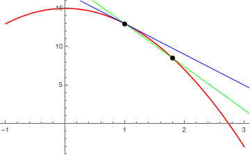
In the OP's example, for the function, we can use the expression f = 15 - 2 x^2 and we can find its derivative with D[f, x] instead of the prime notation. We can also evaluate it at a point x == x0, using ReplaceAll to substitute x0 for x with f /. x -> x0.

f = 15 - 2 x^2;
x0 = 1;
x1 = 1.8;
Show[
 Plot[f, {x, -1, 3}, PlotStyle -> Red],
 Graphics[{
   Blue, InfiniteLine[{x0, f /. x -> x0}, {1, D[f, x] /. x -> x0}],   (* tangent *)
   Green, InfiniteLine[{{x0, f /. x -> x0}, {x1, f /. x -> x1}}],     (* secant *)
   Black, PointSize[Large], Point[{{x0, f /. x -> x0}, {x1, f /. x -> x1}}]
   }]]

Animation

The animation does not seem central to the question. Since the more sensible ways have been done, e.g., using Table or Animate to change x1, here's a different way that wraps the plot above in DynamicModule and animates the figure with Dynamic; the Button bumps x1 a little, which will then approach the point of tangency at x0 with exponentially decaying speed.

DynamicModule[{x0, x1, f},
 f = 15 - 2 x^2;
 x0 = 1;
 x1 = 1.8;
 Column[{
   Button["bump", x1 = x1 + RandomReal[{-1.5, 1.5}]],
   Show[
    Plot[f, {x, -1, 3}, PlotStyle -> Red],
    Graphics[
     Dynamic@{If[Abs[x0 - x1] > 10^-6, x1 = {0.05, 0.95}.{x0, x1}];
       Blue, InfiniteLine[{x0, f /. x -> x0}, {1, D[f, x] /. x -> x0}],
       Green, InfiniteLine[{{x0, f /. x -> x0}, {x1, f /. x -> x1}}],
       Black, PointSize[Large], 
       Point[{{x0, f /. x -> x0}, {x1, f /. x -> x1}}]
       }]]
   }]
 ]

---

Note: The ulterior purpose is that this question is used sometimes as a duplicate of the tangent line question. (For a finite tangent line, sliding a tangent line along a curve is sometimes used as the duplicate.) Most of the questions about tangent lines are complicated by other requirements. This is the oldest question I could find that seemed relevant, and since it has already been linked as a duplicate, I felt this was the best place for this answer.