Efficient way of finding shortest distance between two sets of points in mathematica

Question

I have two sets of 3D points, say

a = RandomReal[1, {10, 3}];
b = RandomReal[1, {10, 3}];

I wanna find the first N pairs that have shortest distance between the two sets, my current approach is to form a NearestFunction from the first list and map it to the second(say, N=3):

f = Nearest[a];
c = Flatten[f/@b, 1];

Then get the result:

N=3;
Transpose[{c[[#]], b[[#]]}]&@ Ordering[Norm/@(c-b),N]

Output={{1st pair},{2nd pair},{3rd pair}}

Question:What is the more efficient way of finding shortest distance pairs of two sets in mathematica?

-edit-

In my actual case, I want to determine the intersection of two shapes(manifolds), but the analytic form of these shapes are not available. I can only compute points on these shapes through numerical process(NDSolve). So I want to use enough many points to approximate these shapes, and use Intersection-like operation to find points that lay approximately on both shapes. The number of points is very large(eg. 10^7), and the points may in high dimensional space(eg. 4D).

Excuse me for my crippled English. I am greatly appreciate any suggestions, thank you very much!

Answer 1

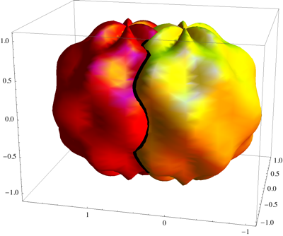
One strength of InterpolatingFunctions is that they can be used just about like any other function. Thus, a more or less analytic approach may be possible. It's hard to say for sure, without seeing your example, but here's a contrived example.

pts1 = Table[{x, y, Sin[x] + Cos[y + 1]}, 
    {x,-10,10}, {y,-10,10}];
f1 = Interpolation[Flatten[pts1, 1]];
pts2 = Table[{x, y, x^2 + y^2 + x + 2 y + 1}, 
    {x,-10,10}, {y,-10,10}];
f2 = Interpolation[Flatten[pts2, 1]];
NMinimize[f2[x, y] - f1[x, y], {x, y}]

Edit

Here's an example that is, perhaps, more in line with your problem. We start with two periodically perturbed spheres - one centered at the origin and one shifted along the y-axis.

pts1 = Flatten[Table[{{p, t}, (1 + 0.1 Sin[6t]Sin[5p])*
  {Sin[p] Cos[t], Sin[p] Sin[t], Cos[p]}},
  {p, 0, Pi, Pi/12}, {t, 0, 2 Pi, Pi/12}], 1];
pts2 = pts1 /. {x_,y_,z_} -> {x,y+0.75,z};

We can interpolate these points and then plot the surfaces parametrically.

f1 = Interpolation[pts1];
f2 = Interpolation[pts2];
surfaces = ParametricPlot3D[{f1[p, t], f2[p, t]}, 
  {p, 0, Pi}, {t, 0, 2 Pi}, MeshStyle -> None, 
  PlotStyle -> {
    Directive[Yellow, Specularity[White, 40]],
    Directive[Red, Specularity[White, 40]]},
  ViewPoint -> {-3, -0.7, 1}]

The question is, where do these two surfaces intersect? The answer is provided by the equation f1[p1,t1]==f2[p2,t2]. Since f1 and f2 are both three dimensional vectors, this represents three equations in four unknowns. We can reduce the number of variables by fixing one and solving for the other three. For example, here is a point that lies on both perturbed spheres and at angle of Pi/4 from the positive z-axis.

Clear[t1, t2, p2];
{t1, t2, p2} = {t1, t2, p2} /. FindRoot[f1[Pi/4, t1] == f2[p2, t2],
  {t1, 2.7, 2.8}, {t2, 3.5, 3.6}, {p2, Pi/4, Pi/4 + 0.1}];
{f1[Pi/4, t1], f2[p2, t2]}

Let's parametrize this process in terms of p1.

Clear[t1, t2, p2];
results = Table[{{p1, t1}, {p2, t2}} /. 
  FindRoot[f1[p1, t1] == f2[p2, t2],
    {t1, 2.7, 2.8}, {t2, 3.5, 3.6}, 
  {p2, p1, p1 + 0.1}], {p1, 0.5, 2.6, 0.1}]; // Quiet

We've suppressed some errors so let's check the results.

test[{pt1_, pt2_}] := Norm[f1 @@ pt1 - f2 @@ pt2];
{#, test[#]} & /@ results

Looks pretty good. Now, with these points, we can parametrize the intersection using an Interpolation, just as we parametrized the surfaces.

intersection = {#[[1]], f1 @@ #} & /@ First /@ results;
p = Interpolation[intersection]

Here's a visualization of the result.

intersectionPic = ParametricPlot3D[p[t], {t, 0.5, 2.8},
  PlotStyle -> Directive[Thickness[0.02], Black]];
Show[{surfaces, intersectionPic}]

Answer 2

I think your approach is good, here is a small improvement:

c = Flatten[
   Developer`ToPackedArray@Table[f[b[[i]], 1], {i, Length[b]}], 1];

edit: shorter code:

c = Join @@ Table[f[b[[i]], 1], {i, Length[b]}]